Creating interpolated tables
A Python interface has been developed that allows the user to run the CompOSE Fortran software in order to create a table of interpolated quantities of their choice, for a given equation of state (EoS). This is particularly useful if the user wishes to use these interpolated values within their own Python scientific analysis.
Available quantities are broadly categorised as follows:
Thermodynamic variables, such as pressure, energy density or entropy etc,
Particle number fractions (electrons, neutrons, protons for example),
Average mass number, proton number and number fraction of a representative nucleus for a given particle set,
Microphysics quantities (for example Dirac or the Landau masses).
Example 1: Cold tables
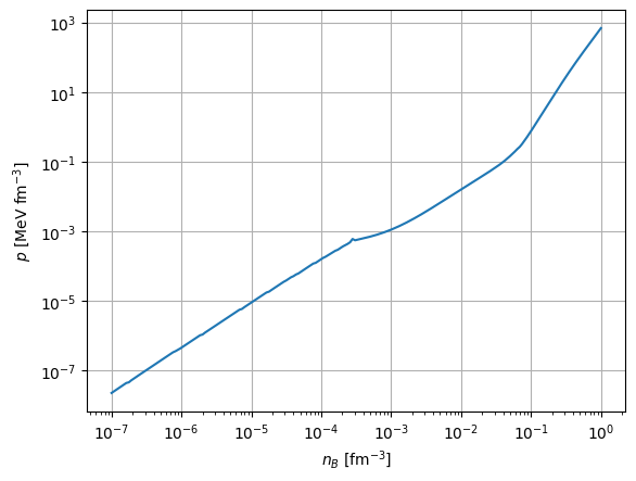
Here, we shall present an example for the case of the EoS PCP(BSk22) where we calculate an interpolated table for the total pressure and the energy density. Furthermore, the interpolation is performed on a grid for baryon number density with the following specifications:
Grid start value: \(1\times{10}^{-7}\) fm\(^{-3}\),
Grid end value: 1.0 fm\(^{-3}\),
200 grid points on a logarithmic scale,
Order 2 (quadratric) interpolation.
First, let’s download a sample EoS:
[1]:
import tempfile

from compytools.download import CompOSEDownloader

# Store in a temporary directory for the purpose of this example.
tmpdir = tempfile.TemporaryDirectory()
getter = CompOSEDownloader.from_eosname('PCP(BSk22)', tmpdir.name)
getter.get()
A summary of the quantities that are available for interpolation for a given EoS, as well as grid parameter information, can be shown using the summary function:
[2]:
from compytools import (
    summarise
)

# Provide the directory to the downloaded tables.
summarise(tmpdir.name)
             Grid parameter information.
┏━━━━━━━━━━━━━━━━┳━━━━━━━━━━━━┳━━━━━━━━━━━━┳━━━━━━━━━┓
┃ Grid Parameter ┃ Minimum    ┃ Maximum    ┃ Unit    ┃
┡━━━━━━━━━━━━━━━━╇━━━━━━━━━━━━╇━━━━━━━━━━━━╇━━━━━━━━━┩
│ t              │ 0.0000e+00 │ 0.0000e+00 │ MeV     │
│ nb             │ 4.6796e-10 │ 1.4922e+00 │ 1 / fm3 │
│ yq             │ 0.0000e+00 │ 0.0000e+00 │         │
└────────────────┴────────────┴────────────┴─────────┘
                         Available thermodynamic quantities.
┏━━━━━━━━━━━━━━━━━┳━━━━━━━━━━━━━━━━━━━━━━━━━━━━━━━━━━━━━━━━━━━━━━━━━┳━━━━━━━━━━━━━━━┓
┃ Quantity Number ┃ Quantity                                        ┃ Unit          ┃
┡━━━━━━━━━━━━━━━━━╇━━━━━━━━━━━━━━━━━━━━━━━━━━━━━━━━━━━━━━━━━━━━━━━━━╇━━━━━━━━━━━━━━━┩
│ 1               │ total pressure                                  │ 1.0 MeV / fm3 │
│ 2               │ total entropy per baryon                        │               │
│ 3               │ shifted baryon chemical potential               │ MeV           │
│ 4               │ charge chemical potential                       │ MeV           │
│ 5               │ lepton chemical potential                       │ MeV           │
│ 6               │ Scaled free energy per baryon                   │               │
│ 7               │ Scaled internal energy per baryon               │               │
│ 8               │ Scaled enthalpy per baryon                      │               │
│ 9               │ Scaled free enthalpy per baryon                 │               │
│ 18              │ isothermal compressibility                      │ fm3 / MeV     │
│ 20              │ Free energy per baryon                          │ MeV           │
│ 21              │ Energy per baryon (with rest mass contribution) │ MeV           │
│ 22              │ enthalpy per baryon                             │ MeV           │
│ 23              │ free enthalpy per baryon                        │ MeV           │
│ 24              │ Energy density                                  │ 1.0 MeV / fm3 │
└─────────────────┴─────────────────────────────────────────────────┴───────────────┘
            Available particle mass fractions.
┏━━━━━━━━━━━━━━━━━┳━━━━━━━━━━━━━━━┳━━━━━━━━━━━━━━━━┳━━━━━━┓
┃ Quantity Number ┃ Quantity Name ┃ Quantity Index ┃ Unit ┃
┡━━━━━━━━━━━━━━━━━╇━━━━━━━━━━━━━━━╇━━━━━━━━━━━━━━━━╇━━━━━━┩
│ 1               │ electron      │ 0              │      │
│ 2               │ muon          │ 1              │      │
│ 3               │ neutron       │ 10             │      │
│ 4               │ proton        │ 11             │      │
└─────────────────┴───────────────┴────────────────┴──────┘
     Nuclear particle indices.
┏━━━━━━━━━━━━━━━━━┳━━━━━━━━━━━━━━━━┓
┃ Quantity number ┃ Particle index ┃
┡━━━━━━━━━━━━━━━━━╇━━━━━━━━━━━━━━━━┩
│ 1               │ 1              │
└─────────────────┴────────────────┘
                                Available microphysics quantities.
┏━━━━━━━━━━━━━━━━━┳━━━━━━━━━━━━━━━━━━━━━━━━━━━━━━━━━━━━━━━━━━━━━━━━━━━━━━┳━━━━━━━━━━━━━━━━┳━━━━━━┓
┃ Quantity Number ┃ Quantity Name                                        ┃ Quantity Index ┃ Unit ┃
┡━━━━━━━━━━━━━━━━━╇━━━━━━━━━━━━━━━━━━━━━━━━━━━━━━━━━━━━━━━━━━━━━━━━━━━━━━╇━━━━━━━━━━━━━━━━╇━━━━━━┩
│ 1               │ effective Landau mass w.r.t particle mass (neutron)  │ 10040          │      │
│ 2               │ effective Landau mass w.r.t particle mass (proton)   │ 11040          │      │
│ 3               │ non-relativistic single particle potential (neutron) │ 10050          │ MeV  │
│ 4               │ non-relativistic single particle potential (proton)  │ 11050          │ MeV  │
│ 5               │ gap (nn (1S0))                                       │ 700060         │ MeV  │
│ 6               │ gap (pp (1S0))                                       │ 702060         │ MeV  │
└─────────────────┴──────────────────────────────────────────────────────┴────────────────┴──────┘
Available quantities can be shown for a given table by using the tables argument. For example, to show available thermodynamic quantities only, we can run summarise(tmpdir.name, tables='thermo'). To show available quantities associated with the thermo and micro tables, we can use summarise(tmpdir.name, tables=['thermo'. 'micro'])
With the exception of the grid parameters, the above tables show the quantity number which, as we will see shortly, will be used to choose the desired quantity that we wish to interpolate. Note also that, for the purposes of this example, the quantity number for the pressure and energy density are 1 and 24, respectively.
First, let’s define the grid for our interpolation:
[3]:
from compytools import (
    GridSettings,
    Interface
)

nbgrid = GridSettings(
    min=1.e-7,
    max=1.0,
    order=2,
    npoints=200,
    logscale=True
)
If the user specifies values for the minimum or maximum grid point values that are outside the allowed range for the given EoS, then they are automatically adjusted to match the limits associated with the input EoS.
Now we can set up the interface to the CompOSE code using the Interface class:
[4]:
interface = Interface(
    # Directory containing the tables
    eospath=tmpdir.name,
    # Grid settings for baryon number density
    nbconfig=nbgrid,
    # Pressure and energy density
    thermo_choice=[1, 24]
)

table = interface.run()
table.pprint()
[10:22:26] INFO File /tmp/tmpjhpajvhu/eos.table created. interface.py:682
    T          nb         Yq      pressure      e
   MeV      1 / fm3              MeV / fm3  MeV / fm3
---------- ---------- ---------- ---------- ----------
0.0000e+00 1.0000e-07 0.0000e+00 2.2354e-08 9.3093e-05
0.0000e+00 1.0844e-07 0.0000e+00 2.4961e-08 1.0095e-04
0.0000e+00 1.1758e-07 0.0000e+00 2.7888e-08 1.0947e-04
0.0000e+00 1.2751e-07 0.0000e+00 3.1148e-08 1.1871e-04
0.0000e+00 1.3826e-07 0.0000e+00 3.4773e-08 1.2872e-04
0.0000e+00 1.4993e-07 0.0000e+00 3.8807e-08 1.3959e-04
0.0000e+00 1.6258e-07 0.0000e+00 4.3314e-08 1.5137e-04
0.0000e+00 1.7629e-07 0.0000e+00 4.5115e-08 1.6414e-04
0.0000e+00 1.9116e-07 0.0000e+00 5.1443e-08 1.7799e-04
       ...        ...        ...        ...        ...
0.0000e+00 4.8241e-01 0.0000e+00 9.4615e+01 5.0363e+02
0.0000e+00 5.2311e-01 0.0000e+00 1.1860e+02 5.5507e+02
0.0000e+00 5.6724e-01 0.0000e+00 1.4831e+02 6.1309e+02
0.0000e+00 6.1510e-01 0.0000e+00 1.8512e+02 6.7881e+02
0.0000e+00 6.6699e-01 0.0000e+00 2.3075e+02 7.5352e+02
0.0000e+00 7.2326e-01 0.0000e+00 2.8741e+02 8.3883e+02
0.0000e+00 7.8428e-01 0.0000e+00 3.5786e+02 9.3667e+02
0.0000e+00 8.5045e-01 0.0000e+00 4.4562e+02 1.0494e+03
0.0000e+00 9.2220e-01 0.0000e+00 5.5509e+02 1.1799e+03
0.0000e+00 1.0000e+00 0.0000e+00 6.9185e+02 1.3318e+03
Length = 200 rows
Not only does this produce an output file containing the interpolated data, but the interface also outputs an astropy table with the chosen quantities on the desired grid. Data can be accessed as follows:
[5]:
import matplotlib.pyplot as plt

plt.figure()
plt.loglog(table['nb'], table['pressure'])
plt.grid()
plt.xlabel(r'$n_{B}$ [fm$^{-3}$]')
plt.ylabel(r'$p$ [MeV fm$^{-3}$]')
[5]:
Text(0, 0.5, '$p$ [MeV fm$^{-3}$]')
For more information about the astropy table functionality, the reader is referred to Reading CompOSE tables.
Choices for the particle number fractions, microphysics and nuclear sets can be similarly specified via the particle_choice, micro_choice and nuclear_choice arguments, respectively.
It is straightforward to modify the settings for our interface instance. For example, if we wish to also include the particle fractions for electrons and muons (quantity numbers 1 and 2, respectively, in the table entitled “Available particle mass fractions”), then we do the following:
[6]:
interface.particle_choice = [1, 2]
table = interface.run()
table.pprint()
[10:22:27] INFO File /tmp/tmpjhpajvhu/eos.table created. interface.py:682
    T          nb         Yq      pressure      e      Y (electron)  Y (muon)
   MeV      1 / fm3              MeV / fm3  MeV / fm3
---------- ---------- ---------- ---------- ---------- ------------ ----------
0.0000e+00 1.0000e-07 0.0000e+00 2.2354e-08 9.3093e-05   4.5161e-01 0.0000e+00
0.0000e+00 1.0844e-07 0.0000e+00 2.4961e-08 1.0095e-04   4.5161e-01 0.0000e+00
0.0000e+00 1.1758e-07 0.0000e+00 2.7888e-08 1.0947e-04   4.5161e-01 0.0000e+00
0.0000e+00 1.2751e-07 0.0000e+00 3.1148e-08 1.1871e-04   4.5161e-01 0.0000e+00
0.0000e+00 1.3826e-07 0.0000e+00 3.4773e-08 1.2872e-04   4.5161e-01 0.0000e+00
0.0000e+00 1.4993e-07 0.0000e+00 3.8807e-08 1.3959e-04   4.5161e-01 0.0000e+00
0.0000e+00 1.6258e-07 0.0000e+00 4.3314e-08 1.5137e-04   4.5166e-01 0.0000e+00
0.0000e+00 1.7629e-07 0.0000e+00 4.5115e-08 1.6414e-04   4.2906e-01 0.0000e+00
0.0000e+00 1.9116e-07 0.0000e+00 5.1443e-08 1.7799e-04   4.3600e-01 0.0000e+00
       ...        ...        ...        ...        ...          ...        ...
0.0000e+00 4.8241e-01 0.0000e+00 9.4615e+01 5.0363e+02   1.1992e-01 8.5977e-02
0.0000e+00 5.2311e-01 0.0000e+00 1.1860e+02 5.5507e+02   1.2879e-01 9.5686e-02
0.0000e+00 5.6724e-01 0.0000e+00 1.4831e+02 6.1309e+02   1.3798e-01 1.0574e-01
0.0000e+00 6.1510e-01 0.0000e+00 1.8512e+02 6.7881e+02   1.4736e-01 1.1601e-01
0.0000e+00 6.6699e-01 0.0000e+00 2.3075e+02 7.5352e+02   1.5676e-01 1.2633e-01
0.0000e+00 7.2326e-01 0.0000e+00 2.8741e+02 8.3883e+02   1.6602e-01 1.3654e-01
0.0000e+00 7.8428e-01 0.0000e+00 3.5786e+02 9.3667e+02   1.7500e-01 1.4650e-01
0.0000e+00 8.5045e-01 0.0000e+00 4.4562e+02 1.0494e+03   1.8356e-01 1.5607e-01
0.0000e+00 9.2220e-01 0.0000e+00 5.5509e+02 1.1799e+03   1.9162e-01 1.6514e-01
0.0000e+00 1.0000e+00 0.0000e+00 6.9185e+02 1.3318e+03   1.9909e-01 1.7364e-01
Length = 200 rows
On the other hand, to adjust the grid settings (for example the minimum grid value and the interpolation order), we proceed as follows:
[7]:
nbgrid.min = 0.08
nbgrid.order = 1

interface.nbconfig = nbgrid
table = interface.run()

table.pprint()
INFO File /tmp/tmpjhpajvhu/eos.table created. interface.py:682
    T          nb         Yq      pressure      e      Y (electron)  Y (muon)
   MeV      1 / fm3              MeV / fm3  MeV / fm3
---------- ---------- ---------- ---------- ---------- ------------ ----------
0.0000e+00 8.0000e-02 0.0000e+00 3.9305e-01 7.5782e+01   3.0688e-02 0.0000e+00
0.0000e+00 8.1022e-02 0.0000e+00 4.0735e-01 7.6755e+01   3.0986e-02 0.0000e+00
0.0000e+00 8.2057e-02 0.0000e+00 4.2226e-01 7.7741e+01   3.1286e-02 0.0000e+00
0.0000e+00 8.3105e-02 0.0000e+00 4.3781e-01 7.8739e+01   3.1589e-02 0.0000e+00
0.0000e+00 8.4166e-02 0.0000e+00 4.5404e-01 7.9751e+01   3.1894e-02 0.0000e+00
0.0000e+00 8.5241e-02 0.0000e+00 4.7097e-01 8.0775e+01   3.2202e-02 0.0000e+00
0.0000e+00 8.6330e-02 0.0000e+00 4.8863e-01 8.1813e+01   3.2513e-02 0.0000e+00
0.0000e+00 8.7433e-02 0.0000e+00 5.0705e-01 8.2865e+01   3.2826e-02 0.0000e+00
0.0000e+00 8.8550e-02 0.0000e+00 5.2627e-01 8.3930e+01   3.3142e-02 0.0000e+00
       ...        ...        ...        ...        ...          ...        ...
0.0000e+00 8.9205e-01 0.0000e+00 5.0722e+02 1.1240e+03   1.8838e-01 1.6149e-01
0.0000e+00 9.0345e-01 0.0000e+00 5.2499e+02 1.1450e+03   1.8963e-01 1.6289e-01
0.0000e+00 9.1499e-01 0.0000e+00 5.4340e+02 1.1664e+03   1.9086e-01 1.6429e-01
0.0000e+00 9.2667e-01 0.0000e+00 5.6245e+02 1.1884e+03   1.9208e-01 1.6567e-01
0.0000e+00 9.3851e-01 0.0000e+00 5.8218e+02 1.2109e+03   1.9329e-01 1.6703e-01
0.0000e+00 9.5050e-01 0.0000e+00 6.0261e+02 1.2339e+03   1.9448e-01 1.6838e-01
0.0000e+00 9.6264e-01 0.0000e+00 6.2376e+02 1.2575e+03   1.9566e-01 1.6972e-01
0.0000e+00 9.7494e-01 0.0000e+00 6.4567e+02 1.2816e+03   1.9682e-01 1.7104e-01
0.0000e+00 9.8739e-01 0.0000e+00 6.6836e+02 1.3064e+03   1.9796e-01 1.7235e-01
0.0000e+00 1.0000e+00 0.0000e+00 6.9186e+02 1.3318e+03   1.9909e-01 1.7364e-01
Length = 200 rows
The above workflow is recommended because this ensures that sanity checking is performed on the new grid settings before we run the interface.
Example 2: Calculating beta equilibrium slices
The interface allows the user to extract beta equilibrium slices from a general purpose EoS. In this example, let’s download RG(SLy4):
[8]:
tmpdir = tempfile.TemporaryDirectory()
getter = CompOSEDownloader.from_eosname('RG(SLy4)', tmpdir.name)
getter.get()
Here, we extract a beta-equilibrium slice for pressure and energy density for the lowest temperature entry for RG(SLy4) of 0.1 MeV. We also define the same baryon number density grid, nbconfig, as described in Example 1.
[9]:
nbconfig = GridSettings(
    min=1.e-7,
    max=1,
    order=2,
    npoints=200,
    logscale=True
)
For the temperature grid, min and max will be equal and so it is not neccessary to provide the other arguments to GridSettings:
[10]:
tconfig = GridSettings(min=0.1, max=0.1)
Pressure along the beta-equilibrium slice will be computed as a function of the charge number fraction, so we will just need to supply the corresponding interpolation order, for example:
[11]:
yqconfig = GridSettings(order=2)
We then set up our interface instance, specifying the above grid settings for temperature, baryon number density and charge fraction. We also need to set the slice_betaeq=True:
[12]:
interface = Interface(
    eospath=tmpdir.name,
    nbconfig=nbconfig,
    tconfig=tconfig,
    yqconfig=yqconfig,
    thermo_choice=[1],
    slice_betaeq=True
)

table = interface.run()
table.pprint()
[10:24:16] INFO File /tmp/tmpaoc9n1w1/eos.table created. interface.py:682
    T          nb         Yq      pressure
   MeV      1 / fm3              MeV / fm3
---------- ---------- ---------- ----------
1.0000e-01 1.0000e-07 4.4841e-01 2.2335e-08
1.0000e-01 1.0844e-07 4.4794e-01 2.4908e-08
1.0000e-01 1.1758e-07 4.4744e-01 2.7765e-08
1.0000e-01 1.2751e-07 4.4696e-01 3.0860e-08
1.0000e-01 1.3826e-07 4.4651e-01 3.4168e-08
1.0000e-01 1.4993e-07 4.4595e-01 3.7969e-08
1.0000e-01 1.6258e-07 4.4517e-01 4.2460e-08
1.0000e-01 1.7629e-07 4.4429e-01 4.7518e-08
1.0000e-01 1.9116e-07 4.4356e-01 5.2773e-08
       ...        ...        ...        ...
1.0000e-01 4.8241e-01 5.7217e-02 6.2034e+01
1.0000e-01 5.2311e-01 5.7471e-02 7.8872e+01
1.0000e-01 5.6724e-01 5.7882e-02 9.9966e+01
1.0000e-01 6.1510e-01 5.8392e-02 1.2641e+02
1.0000e-01 6.6699e-01 5.9205e-02 1.5981e+02
1.0000e-01 7.2326e-01 6.0457e-02 2.0223e+02
1.0000e-01 7.8428e-01 6.2182e-02 2.5592e+02
1.0000e-01 8.5045e-01 6.4509e-02 3.2280e+02
1.0000e-01 9.2220e-01 6.7425e-02 4.0616e+02
1.0000e-01 1.0000e+00 7.1424e-02 5.1083e+02
Length = 200 rows
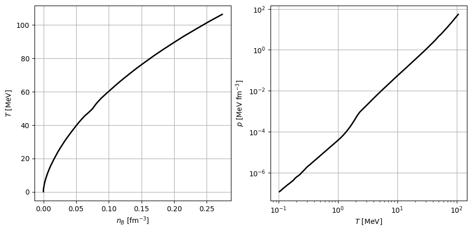
Example 3 - Slices in fixed entropy
In this example, we extract a slice for an entropy per baryon of 4, for a fixed charge number fraction of 0.1. The grid configurations for the charge number fraction and temperature are now:
[13]:
# Charge fraction is fixed so the minimum and maximum values are the same
yqconfig = GridSettings(min=0.1, max=0.1)

# Quantities are written on temperature grid, so just provide the interpolation order
tconfig = GridSettings(order=3)
To supply the entropy per baryon, we use the slice_fixed_entropy_per_baryon option:
[14]:
interface = Interface(
    eospath=tmpdir.name,
    thermo_choice=[1],
    slice_fixed_entropy_per_baryon=4,
    nbconfig=nbconfig,
    yqconfig=yqconfig,
    tconfig=tconfig
)

table = interface.run()
print(table)
[10:24:23] INFO File /tmp/tmpaoc9n1w1/eos.table created. interface.py:682
    T          nb         Yq      pressure
   MeV      1 / fm3              MeV / fm3
---------- ---------- ---------- ----------
1.0337e-01 8.9074e-07 1.0000e-01 1.1814e-07
1.0917e-01 9.6588e-07 1.0000e-01 1.3376e-07
1.1391e-01 1.0474e-06 1.0000e-01 1.5004e-07
1.1939e-01 1.1357e-06 1.0000e-01 1.6897e-07
1.2553e-01 1.2316e-06 1.0000e-01 1.9084e-07
1.3220e-01 1.3355e-06 1.0000e-01 2.1590e-07
1.3943e-01 1.4481e-06 1.0000e-01 2.4461e-07
1.4739e-01 1.5703e-06 1.0000e-01 2.7778e-07
1.5654e-01 1.7028e-06 1.0000e-01 3.1651e-07
       ...        ...        ...        ...
7.0820e+01 1.3201e-01 1.0000e-01 1.3390e+01
7.4233e+01 1.4315e-01 1.0000e-01 1.5620e+01
7.7684e+01 1.5522e-01 1.0000e-01 1.8206e+01
8.1384e+01 1.6832e-01 1.0000e-01 2.1267e+01
8.5151e+01 1.8252e-01 1.0000e-01 2.4831e+01
8.9074e+01 1.9792e-01 1.0000e-01 2.9015e+01
9.3216e+01 2.1461e-01 1.0000e-01 3.3952e+01
9.7391e+01 2.3272e-01 1.0000e-01 3.9694e+01
1.0186e+02 2.5235e-01 1.0000e-01 4.6514e+01
1.0640e+02 2.7364e-01 1.0000e-01 5.4477e+01
Length = 157 rows
[15]:
plt.figure(figsize=(11, 5))
plt.subplot(121)
plt.plot(table['nb'], table['T'], '-k', linewidth=2)
plt.xlabel(r'$n_{B}$ [fm$^{-3}$]')
plt.ylabel(r'$T$ [MeV]')
plt.grid()

plt.subplot(122)
plt.loglog(table['T'], table['pressure'], '-k', linewidth=2)
plt.xlabel(r'$T$ [MeV]')
plt.ylabel(r'$p$ [MeV fm$^{-3}$]')
plt.grid()
Example 4 - Arbitrary grid parameters
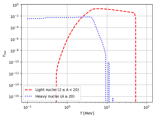
In this example, we will create an interpolated table of the nuclear mass fraction \(Y_{\mathrm{nuc}}\) for \(n_{B}=0.01\) fm\(^{-3}\) and \(Y_{\mathrm{q}}=0.3\). We will consider a grid in temperature between 0 and 100 MeV with 100 points on a logarithmic scale, with second-order interpolation. Let’s examine which nuclear particle sets are available for this EoS:
[16]:
summarise(tmpdir.name, tables='compo')
            Available particle mass fractions.
┏━━━━━━━━━━━━━━━━━┳━━━━━━━━━━━━━━━┳━━━━━━━━━━━━━━━━┳━━━━━━┓
┃ Quantity Number ┃ Quantity Name ┃ Quantity Index ┃ Unit ┃
┡━━━━━━━━━━━━━━━━━╇━━━━━━━━━━━━━━━╇━━━━━━━━━━━━━━━━╇━━━━━━┩
│ 1               │ neutron       │ 10             │      │
│ 2               │ proton        │ 11             │      │
│ 3               │ deuteron 2H   │ 2001           │      │
│ 4               │ triton 3H     │ 3001           │      │
│ 5               │ helion 3He    │ 3002           │      │
│ 6               │ alpha 4He     │ 4002           │      │
│ 7               │ electron      │ 0              │      │
└─────────────────┴───────────────┴────────────────┴──────┘
     Nuclear particle indices.
┏━━━━━━━━━━━━━━━━━┳━━━━━━━━━━━━━━━━┓
┃ Quantity number ┃ Particle index ┃
┡━━━━━━━━━━━━━━━━━╇━━━━━━━━━━━━━━━━┩
│ 1               │ 1              │
│ 2               │ 2              │
└─────────────────┴────────────────┘
We will plot \(Y_{nuc}\) for both particle indices. The data sheet indicates that set 1 corresponds to light nuclei (\(2\leq{A}<20\)) while set 2 corresponds to heavy nuclei (\(A\geq{20}\)). The grid settings are:
[17]:
tconfig = GridSettings(
    min=0,
    max=100,
    order=2,
    npoints=100,
    logscale=True
)

nbconfig = GridSettings(min=0.01, max=0.01)
yqconfig = GridSettings(min=0.3, max=0.3)
while for the interface we have:
[18]:
interface = Interface(
    eospath=tmpdir.name,
    nbconfig=nbconfig,
    tconfig=tconfig,
    yqconfig=yqconfig,
    nuclear_choice=[1, 2]
)

table = interface.run()
table.pprint(max_width=-1)
[10:24:28] INFO File /tmp/tmpaoc9n1w1/eos.table created. interface.py:682
    T          nb         Yq     Ynuc (set #1) Aav (set #1) Zav (set #1) Nav (set #1) Ynuc (set #2) Aav (set #2) Zav (set #2) Nav (set #2)
   MeV      1 / fm3
---------- ---------- ---------- ------------- ------------ ------------ ------------ ------------- ------------ ------------ ------------
1.0001e-01 1.0000e-02 3.0000e-01    0.0000e+00   0.0000e+00   0.0000e+00   0.0000e+00    3.4063e-03   2.0694e+02   6.2221e+01   1.4472e+02
1.0724e-01 1.0000e-02 3.0000e-01    0.0000e+00   0.0000e+00   0.0000e+00   0.0000e+00    3.4088e-03   2.0680e+02   6.2221e+01   1.4458e+02
1.1499e-01 1.0000e-02 3.0000e-01    0.0000e+00   0.0000e+00   0.0000e+00   0.0000e+00    3.4116e-03   2.0666e+02   6.2221e+01   1.4443e+02
1.2330e-01 1.0000e-02 3.0000e-01    0.0000e+00   0.0000e+00   0.0000e+00   0.0000e+00    3.4146e-03   2.0650e+02   6.2221e+01   1.4428e+02
1.3221e-01 1.0000e-02 3.0000e-01    0.0000e+00   0.0000e+00   0.0000e+00   0.0000e+00    3.4177e-03   2.0633e+02   6.2221e+01   1.4411e+02
1.4176e-01 1.0000e-02 3.0000e-01    0.0000e+00   0.0000e+00   0.0000e+00   0.0000e+00    3.4209e-03   2.0617e+02   6.2230e+01   1.4394e+02
1.5201e-01 1.0000e-02 3.0000e-01    0.0000e+00   0.0000e+00   0.0000e+00   0.0000e+00    3.4262e-03   2.0587e+02   6.2177e+01   1.4369e+02
1.6299e-01 1.0000e-02 3.0000e-01    0.0000e+00   0.0000e+00   0.0000e+00   0.0000e+00    3.4363e-03   2.0526e+02   6.1978e+01   1.4328e+02
1.7477e-01 1.0000e-02 3.0000e-01    0.0000e+00   0.0000e+00   0.0000e+00   0.0000e+00    3.4475e-03   2.0459e+02   6.1752e+01   1.4284e+02
       ...        ...        ...           ...          ...          ...          ...           ...          ...          ...          ...
5.3367e+01 1.0000e-02 3.0000e-01    3.9341e-03   2.4792e-01   1.2133e-01   1.2659e-01    0.0000e+00   0.0000e+00   0.0000e+00   0.0000e+00
5.7224e+01 1.0000e-02 3.0000e-01    0.0000e+00   0.0000e+00   0.0000e+00   0.0000e+00    0.0000e+00   0.0000e+00   0.0000e+00   0.0000e+00
6.1360e+01 1.0000e-02 3.0000e-01    0.0000e+00   0.0000e+00   0.0000e+00   0.0000e+00    0.0000e+00   0.0000e+00   0.0000e+00   0.0000e+00
6.5794e+01 1.0000e-02 3.0000e-01    0.0000e+00   0.0000e+00   0.0000e+00   0.0000e+00    0.0000e+00   0.0000e+00   0.0000e+00   0.0000e+00
7.0548e+01 1.0000e-02 3.0000e-01    0.0000e+00   0.0000e+00   0.0000e+00   0.0000e+00    0.0000e+00   0.0000e+00   0.0000e+00   0.0000e+00
7.5647e+01 1.0000e-02 3.0000e-01    0.0000e+00   0.0000e+00   0.0000e+00   0.0000e+00    0.0000e+00   0.0000e+00   0.0000e+00   0.0000e+00
8.1113e+01 1.0000e-02 3.0000e-01    0.0000e+00   0.0000e+00   0.0000e+00   0.0000e+00    0.0000e+00   0.0000e+00   0.0000e+00   0.0000e+00
8.6975e+01 1.0000e-02 3.0000e-01    0.0000e+00   0.0000e+00   0.0000e+00   0.0000e+00    0.0000e+00   0.0000e+00   0.0000e+00   0.0000e+00
9.3260e+01 1.0000e-02 3.0000e-01    0.0000e+00   0.0000e+00   0.0000e+00   0.0000e+00    0.0000e+00   0.0000e+00   0.0000e+00   0.0000e+00
1.0000e+02 1.0000e-02 3.0000e-01    0.0000e+00   0.0000e+00   0.0000e+00   0.0000e+00    0.0000e+00   0.0000e+00   0.0000e+00   0.0000e+00
Length = 100 rows
[19]:
plt.figure()
plt.loglog(table['T'], table['Ynuc (set #1)'], '--r', linewidth=2, label=r'Light nuclei ($2\leq{A}<20$)')
plt.loglog(table['T'], table['Ynuc (set #2)'], ':b', linewidth=2, label=r'Heavy nuclei ($A\geq{20}$)')
plt.xlabel(r'$T$ [MeV]')
plt.ylabel(r'$Y_{nuc}$')

plt.legend()
plt.grid()