Creating tables in the CompOSE format
This section describes how a contributor can provide a cold equation of state (EoS) in the CompOSE format. The following tables are mandatory:
eos.[t,nb,yq]: Grid parameter files in temperature, baryon number density and charge fraction, respectively,eos.thermo: Contains the thermodynamic quantities,eos.init: Not strictly a table, but this correctly initialises theCompOSEFortran code for creating interpolated tables.
The following tables are optional:
eos.compo: Holds particle mass fractions and nuclear data,eos.micro: Contains microphysics quantities,eos.mr: Neutron star static properties (for example the mass, radius and tidal deformability).
See Section 4.2 in the CompOSE manual at https://compose.obspm.fr/manual for further information.
To describe this functionality we consider, as a simple example, a Fermi gas consisting of only protons, neutrons and electrons in beta equilibrium. The aim is to convert the output calculated from this model into CompOSE tables.
Functionality to write general purpose tables will be provided in a future release of ComPyTools.
Description of the data
We have created a file that contains the following data:
Column |
Quantity |
Units |
|---|---|---|
1 |
Baryon number density |
fm\(^{-3}\) |
2 |
Pressure |
dyn cm\(^{-2}\) |
3 |
Neutron chemical potential |
erg |
4 |
Proton chemical potential |
erg |
4 |
Electron chemical potential |
erg |
5 |
Mass energy density |
gm cm\(^{-3}\) |
6 |
Electron num. fraction |
|
7 |
Proton num. fraction |
|
8 |
Neutron num. fraction |
We start by creating the mandatory CompOSE tables eos.[t,nb,yq] and eos.thermo, followed by the optional tables eos.compo, eos.micro and eos.mr.
The toy model data is created by the script https://gitlab.in2p3.fr/lpc-caen/compytools/-/blob/main/src/Tools/Scr_WriteEoSToyData.py.
Let’s load our EoS data:
[1]:
import os
import numpy as np

eos_path = os.path.join('../../', 'tests', 'inputs', 'FermiGas')
eos_table = os.path.join(eos_path, 'eos_fermi_gas.dat')

nbgrid, p, mun, mup, mue, eps, Ye, Yp, Yn = np.loadtxt(
    eos_table,
    unpack=True
)
Grid parameter files (eos.[t,nb,yq])
See Section 4.2.7 in the CompOSE https://compose.obspm.fr/manual for further information about the grid parameter files.
There are two steps to create a given table:
Feed the data into a “data” interface and provide units. This allows the code to perform sanity checking on the units, perform conversions if necessary and compute automatically any additional quantities expected by
CompOSE,Feed that data into a “table” interface. This stores the data in tabular form, allowing the user to view and inspect the data. This tabular form also makes it possible to write the data to file further down the line.
[2]:
from compytools import (
    Grid,
    GridData
)

# Load useful units for our input data
from compytools.constants import (
  DIMENSIONLESS,
  MEV,
  PERCM3,
  PERFM3
)
First step: feed in the grid points into the GridData class. For cold tables there is only a single value for temperature and charge fraction, which are both zero:
[3]:
grid_data = GridData(
    # Temperature grid points in MeV
    t=np.array([0.0]) << MEV,
    # Baryon number density in 1/cm^3
    nb=nbgrid << PERCM3,
    # Charge fraction (no units)
    yq=np.array([0.0]) << DIMENSIONLESS
)
Here and elsewhere, it is mandatory to provide units even if they are already in the units as required by CompOSE. This not only allows ComPyTools to perform sanity checking on the input data, but it also allows units to be added to the table’s metadata.
Second Step: create the table via the Grid class. Note how the values for the baryon number density have automatically been converted into fm\(^{-3}\), as required by CompOSE.
[4]:
grid_params = Grid.from_dataset(grid_data)
grid_params.nb.grid_points
[4]:
Thermodynamic quantities (eos.thermo)
A similar procedure as described above the grid parameter data is followed for the remaining tables.
See Section 4.2.2 in the CompOSE https://compose.obspm.fr/manual for further information about the table for thermodynamic quantities.
Here we provide the data for the eos.thermo table.
[5]:
from compytools import (
    Nucleons,
    Thermo,
    ThermoData
)

from compytools.constants import (
    CLIGHT_CGS_SQ,
    DYN_PER_CM2,
    ERG,
    GRAM,
    G_PER_CM3,
    KELVIN,
    MEV,
    MEV_PER_FM3
)
The first line of the eos.thermo file contains the following information:
The neutron and proton masses,
An integer that indicates whether leptons are considered in the EoS.
We provide this information via the Nucleons interface. Note how the nucleon masses have been automatically converted.
[6]:
mn = 1.6749286e-24 << GRAM
mp = 1.6726231e-24 << GRAM

nucleons = Nucleons(mn=mn, mp=mp, has_leptons=1)

print(nucleons)
Nucleons(has_leptons=1, mn=<Quantity 939.56603867 MeV>, mp=<Quantity 938.27274802 MeV>)
Provide the thermodynamic data. Here, we will provide the square of the sound speed (in units of the square of the speed of light) as an additional thermodynamic quantity.
[7]:
# astropy.units allows the user to easily convert units via the to() method,
# in this case into MeV/fm^3 for the pressure and the energy density. The <<
# syntax allows you to specify units for a given quantity.
total_pressure = (p << DYN_PER_CM2).to(MEV_PER_FM3)
energy_density = (eps * CLIGHT_CGS_SQ * G_PER_CM3).to(MEV_PER_FM3)

cs2 = np.gradient(total_pressure, energy_density, edge_order=2)

# Additional thermodynamic quantites should be passed as a dictionary
extra_thermo = {
    'cs2': cs2
}
Now provide the thermodynamic data. For the case of a cold EoS, the entropy density and the lepton chemical potential are zero.
[8]:
# TO-DO: check how the charge and baryon chemical potentials are calculated
thermo_data = ThermoData(
    # Provide the grid parameter provided above
    grid_params=grid_params,
    # Provide the nucleon masses provided above.
    nucleons=nucleons,
    pressure=total_pressure,
    entropy_density=np.zeros(nbgrid.size) << (ERG / KELVIN) * PERCM3,
    baryon_chemical_potential=mun << ERG,
    charge_chemical_potential=mup - mue << ERG,
    lepton_chemical_potential=np.zeros(nbgrid.size) << MEV,
    free_energy_density=eps << G_PER_CM3,
    internal_energy_density=eps << G_PER_CM3,
    # Additional quantities provided via the `Qextra` argument.
    # This can be omitted otherwise.
    Qextra=extra_thermo
)

# Now create the thermo table
thermo = Thermo.from_dataset(thermo_data)
The data, as well as the associated metadata, can be accessed with the respective methods:
[9]:
thermo.pprint(max_width=-1)
thermo.info
 iT jnB kYq     Q1         Q2         Q3         Q4         Q5          Q6          Q7     Nextra  Qextra_1
               MeV
--- --- --- ---------- ---------- ---------- ---------- ---------- ----------- ----------- ------ ----------
  0   1   1 3.6444e-02 0.0000e+00 3.1046e-08 9.9778e-01 0.0000e+00 -4.9557e-01 -4.9557e-01      1 1.1977e-04
  0   2   1 3.8890e-02 0.0000e+00 3.1046e-08 9.9776e-01 0.0000e+00 -4.9557e-01 -4.9557e-01      1 1.2848e-04
  0   3   1 4.1548e-02 0.0000e+00 3.1046e-08 9.9773e-01 0.0000e+00 -4.9556e-01 -4.9556e-01      1 1.3294e-04
  0   4   1 4.3869e-02 0.0000e+00 3.1046e-08 9.9771e-01 0.0000e+00 -4.9556e-01 -4.9556e-01      1 1.3986e-04
  0   5   1 4.6749e-02 0.0000e+00 3.1046e-08 9.9769e-01 0.0000e+00 -4.9555e-01 -4.9555e-01      1 1.5121e-04
  0   6   1 4.9650e-02 0.0000e+00 3.1046e-08 9.9767e-01 0.0000e+00 -4.9554e-01 -4.9554e-01      1 1.5845e-04
  0   7   1 5.2653e-02 0.0000e+00 3.1046e-08 9.9764e-01 0.0000e+00 -4.9554e-01 -4.9554e-01      1 1.6603e-04
  0   8   1 5.5691e-02 0.0000e+00 3.1046e-08 9.9761e-01 0.0000e+00 -4.9553e-01 -4.9553e-01      1 1.7542e-04
  0   9   1 5.9023e-02 0.0000e+00 3.1046e-08 9.9758e-01 0.0000e+00 -4.9552e-01 -4.9552e-01      1 1.8614e-04
... ... ...        ...        ...        ...        ...        ...         ...         ...    ...        ...
  0 191   1 4.7540e+01 0.0000e+00 3.9841e-01 7.1313e-01 0.0000e+00 -4.1084e-01 -4.1084e-01      1 1.2279e-01
  0 192   1 5.0677e+01 0.0000e+00 4.2497e-01 6.9984e-01 0.0000e+00 -4.0474e-01 -4.0474e-01      1 1.2856e-01
  0 193   1 5.3989e+01 0.0000e+00 4.5306e-01 6.8631e-01 0.0000e+00 -3.9825e-01 -3.9825e-01      1 1.3442e-01
  0 194   1 5.7483e+01 0.0000e+00 4.8275e-01 6.7257e-01 0.0000e+00 -3.9134e-01 -3.9134e-01      1 1.4037e-01
  0 195   1 6.1165e+01 0.0000e+00 5.1412e-01 6.5863e-01 0.0000e+00 -3.8398e-01 -3.8398e-01      1 1.4638e-01
  0 196   1 6.5043e+01 0.0000e+00 5.4722e-01 6.4454e-01 0.0000e+00 -3.7615e-01 -3.7615e-01      1 1.5245e-01
  0 197   1 6.9125e+01 0.0000e+00 5.8215e-01 6.3031e-01 0.0000e+00 -3.6783e-01 -3.6783e-01      1 1.5855e-01
  0 198   1 7.3416e+01 0.0000e+00 6.1897e-01 6.1598e-01 0.0000e+00 -3.5900e-01 -3.5900e-01      1 1.6467e-01
  0 199   1 7.7925e+01 0.0000e+00 6.5777e-01 6.0156e-01 0.0000e+00 -3.4962e-01 -3.4962e-01      1 1.7079e-01
  0 200   1 8.2660e+01 0.0000e+00 6.9862e-01 5.8709e-01 0.0000e+00 -3.3967e-01 -3.3967e-01      1 1.7733e-01
Length = 200 rows
[9]:
<Thermo length=200>
  name    dtype  unit format                    description                      class
-------- ------- ---- ------ -------------------------------------------------- --------
      iT   int32          %d                             Temperature grid point   Column
     jnB   int32          %d                     Baryon num. density grid point   Column
     kYq   int32          %d                    Charge num. fraction grid point   Column
      Q1 float32  MeV   %.4e       pressure divided by baryon num. density p/nb Quantity
      Q2 float32        %.4e                            entropy per baryon s/nb Quantity
      Q3 float32        %.4e scaled and shifted baryon chem. potential mub/mn-1 Quantity
      Q4 float32        %.4e            scaled charge chemical potential muq/mn Quantity
      Q5 float32        %.4e  scaled effective lepton chemical potential mul/mn Quantity
      Q6 float32        %.4e      scaled free energy per baryon f/(nb x mn) - 1 Quantity
      Q7 float32        %.4e  scaled internal energy per baryon e/(nb x mn) - 1 Quantity
  Nextra   int32          %d                num. extra thermodynamic quantities   Column
Qextra_1 float32        %.4e     Additional thermodynamic quantity with index 1 Quantity
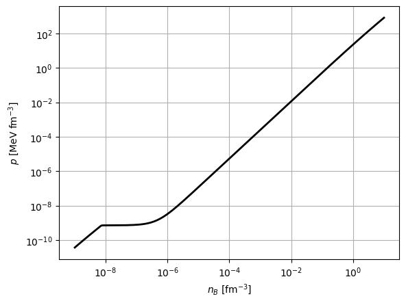
Data can be accessed (for example for plotting) as described in the Section Reading CompOSE tables.
[10]:
import matplotlib.pyplot as plt

plt.figure()

nb = grid_params.nb.grid_points
pressure = nb * thermo['Q1']
plt.loglog(nb, pressure, '-k', linewidth=2)

plt.xlabel(r'$n_{B}$ [fm$^{-3}$]')
plt.ylabel(r'$p$ [MeV fm$^{-3}$]')
plt.grid()
Composition (eos.compo)
See Section 4.2.3 in the CompOSE https://compose.obspm.fr/manual for further information about the table for the composition of matter.
[11]:
from compytools import (
    Compo,
    CompoData,
    NuclearSet
)
First, lets provide the number fractions for each of the particles that are considered by our model. We use a Python dictionary to provide these fractions, where the key for each entry has the form Y (<particle_name>) and <particle_name should be replaced by the name of the particle under consideration. The list of available particle names can be listed by running the following function:
[12]:
from compytools import show_particles

show_particles()
    Available CompOSE particles.
┏━━━━━━━━━━━━━━━━┳━━━━━━━━━━━━━━━━━━┓
┃ Particle Index ┃ Particle Name    ┃
┡━━━━━━━━━━━━━━━━╇━━━━━━━━━━━━━━━━━━┩
│ 0              │ electron         │
│ 1              │ muon             │
│ 10             │ neutron          │
│ 11             │ proton           │
│ 20             │ Delta^-          │
│ 21             │ Delta^0          │
│ 22             │ Delta^+          │
│ 23             │ Delta^++         │
│ 100            │ Lambda           │
│ 110            │ Sigma^-          │
│ 111            │ Sigma^0          │
│ 112            │ Sigma^+          │
│ 120            │ Xi^-             │
│ 121            │ Xi^0             │
│ 200            │ omega            │
│ 210            │ sigma            │
│ 220            │ eta              │
│ 230            │ eta^prime        │
│ 300            │ rho^-            │
│ 301            │ rho^0            │
│ 302            │ rho^+            │
│ 310            │ delta^-          │
│ 311            │ delta^0          │
│ 312            │ delta^+          │
│ 320            │ pi^-             │
│ 321            │ pi^0             │
│ 322            │ pi^+             │
│ 400            │ phi              │
│ 410            │ sigma_s          │
│ 420            │ K^-              │
│ 421            │ K^0              │
│ 422            │ Kbar^0           │
│ 423            │ Kbar^+           │
│ 424            │ K^- (thermal)    │
│ 425            │ K^- (condensate) │
│ 500            │ u quark          │
│ 501            │ d quark          │
│ 502            │ s quark          │
│ 600            │ photon           │
│ 700            │ nn (1S0)         │
│ 701            │ np (1S0)         │
│ 702            │ pp (1S0)         │
│ 703            │ np (3S1)         │
│ 2001           │ deuteron 2H      │
│ 3001           │ triton 3H        │
│ 3002           │ helion 3He       │
│ 4002           │ alpha 4He        │
└────────────────┴──────────────────┘
This table corresponds to Tables 3.3, 3.4 and 3.5 in the CompOSE manual https://compose.obspm.fr/manual.
[13]:
particle_fractions = {
    'Y (electron)': Ye << DIMENSIONLESS,
    'Y (proton)': Yp << DIMENSIONLESS,
    'Y (neutron)': Yn << DIMENSIONLESS
}
We can also provide, for an index \(I_{i}\) that specifies a group of nuclei \(\mathcal{M}_{I_{i}}\), an average mass number Aav, proton number Zav and combined fraction Ynuc via the NuclearSet interface as follows:
[14]:
nuclear_sets = {
    1: NuclearSet(
        Aav=np.zeros(nbgrid.size) << DIMENSIONLESS,
        Zav=np.zeros(nbgrid.size) << DIMENSIONLESS,
        Ynuc=np.zeros(nbgrid.size) << DIMENSIONLESS
    )
}
Alternatively, if no nuclear sets are to be provided by the user, one can specify nuclear_sets=None.
Here, the dictionary key gives the value \(I_{i}\) for a given nuclear set. Note that, since our model does not consider nuclei, we have simply provided arrays filled with zeros for each quantity.
Next, provide the phase indices that define the neutron star structure. For our simple model, we define the interger 1 to indicate that our EoS consists entirely of a gas:
[15]:
Iphase = np.full(nbgrid.size, 1)
Now provide the data via the CompoData interface and then create the data table with the Compo class:
[16]:
compo_data = CompoData(
    grid_params=grid_params,
    Iphase=Iphase,
    particle_fractions=particle_fractions,
    nuclear_sets=nuclear_sets
)

compo = Compo.from_dataset(compo_data)
Microphysics (eos.micro)
See Section 4.2.4 in the CompOSE manual https://compose.obspm.fr/manual for further information about the microphysics table.
The microphysics quantities are provided via dictionary where the keys takes the form <quantity> (<particle_name>). The available particle names can be listed using the aforementioned function show_particles(), while the list of available microphysics quantities can be shown with:
[17]:
from compytools import show_microphysics

show_microphysics()
                                    Available CompOSE microphysics quantities.
┏━━━━━━━━━━━━━━━━━━━━┳━━━━━━━━━━━━━━━━━━━━━━━━━┳━━━━━━━━━━━━━━━━━━━━━━━━━━━━━━━━━━━━━━━━━━━━━━━━━━━━━━━━━━━┳━━━━━━┓
┃ Microphysics Index ┃ Microphysics Quantity   ┃ Description                                               ┃ Unit ┃
┡━━━━━━━━━━━━━━━━━━━━╇━━━━━━━━━━━━━━━━━━━━━━━━━╇━━━━━━━━━━━━━━━━━━━━━━━━━━━━━━━━━━━━━━━━━━━━━━━━━━━━━━━━━━━╇━━━━━━┩
│ 40                 │ m_L/m (<particle_name>) │ effective Landau mass w.r.t particle mass                 │      │
│                    │                         │ (<particle_name>)                                         │      │
│ 41                 │ m_D/m (<particle_name>) │ effective Dirac mass w.r.t particle mass                  │      │
│                    │                         │ (<particle_name>)                                         │      │
│ 50                 │ U (<particle_name>)     │ non-relativistic single particle potential                │ MeV  │
│                    │                         │ (<particle_name>)                                         │      │
│ 51                 │ V (<particle_name>)     │ relativistic vector self-energy (<particle_name>)         │ MeV  │
│ 52                 │ S (<particle_name>)     │ relativistic scalar self-energy (<particle_name>)         │ MeV  │
│ 60                 │ Delta (<particle_name>) │ gap (<particle_name>)                                     │ MeV  │
└────────────────────┴─────────────────────────┴───────────────────────────────────────────────────────────┴──────┘
This table corresponds to Table 7.5 in the CompOSE manual https://compose.obspm.fr/manual.
[18]:
microphysics = {
    'm_L/m (proton)': np.full(nbgrid.size, 1) << DIMENSIONLESS,
    'm_L/m (neutron)': np.full(nbgrid.size, 1) << DIMENSIONLESS
}
In our simple model, we simply provide a value of one for each quantity, for each grid point. Next,
[19]:
from compytools import (
    Micro,
    MicroData
)

micro_data = MicroData(
    grid_params=grid_params,
    microphysics=microphysics
)

micro = Micro.from_dataset(micro_data)
Neutron star properties
See Section 4.2.6 in the CompOSE manual https://compose.obspm.fr/manual for further information about the neutron star properties table.
We have prepared data for the neutron star properties, calculated from a TOV solver, for our toy EoS. The file contains the following quantities:
Column |
Quantity |
Units |
|---|---|---|
1 |
Mass |
grams |
2 |
Radius |
cm |
3 |
Tidal deformability |
The toy TOV data is created by the script https://gitlab.in2p3.fr/lpc-caen/compytools/-/blob/main/src/Tools/Scr_WriteEoSToyData.py.
Let’s load the data:
[20]:
tov_data = os.path.join(eos_path, 'tov_fermi_gas.dat')
mass, radius, Lambda = np.loadtxt(tov_data, unpack=True)
Feed in the data to the NeutronStarData class and create the table via NeutronStar:
[21]:
from compytools import (
    NeutronStarData,
    NeutronStar
)

from compytools.constants import (
    GRAM,
    CM
)

ns_data = NeutronStarData(
    mass=mass << GRAM,
    radius=radius << CM,
    Lambda=Lambda << DIMENSIONLESS,
)

mr = NeutronStar.from_dataset(ns_data)
mr.pprint()
  radius      mass      Lambda
    km      solMass
---------- ---------- ----------
2.0685e+01 2.9813e-01 1.9306e+05
2.0075e+01 3.1766e-01 1.3117e+05
1.9480e+01 3.3793e-01 8.9456e+04
1.8890e+01 3.5889e-01 6.1253e+04
1.8315e+01 3.8047e-01 4.2125e+04
1.7750e+01 4.0256e-01 2.9108e+04
1.7195e+01 4.2503e-01 2.0216e+04
1.6650e+01 4.4776e-01 1.4119e+04
1.6115e+01 4.7060e-01 9.9185e+03
       ...        ...        ...
1.0495e+01 6.8004e-01 2.6371e+02
1.0100e+01 6.8648e-01 2.0735e+02
9.7200e+00 6.9070e-01 1.6482e+02
9.3500e+00 6.9271e-01 1.3246e+02
8.9950e+00 6.9251e-01 1.0765e+02
8.6550e+00 6.9020e-01 8.8476e+01
8.3300e+00 6.8587e-01 7.3553e+01
8.0200e+00 6.7969e-01 6.1855e+01
7.7200e+00 6.7179e-01 5.2623e+01
7.4400e+00 6.6229e-01 4.5294e+01
Length = 30 rows
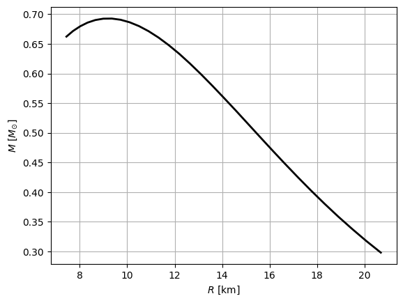
[22]:
# Plot the mass-radius curve
plt.plot(mr['radius'], mr['mass'], '-k', linewidth=2)
plt.xlabel(r'$R$ [km]')
plt.ylabel(r'$M$ [$M_{\odot}$]')

plt.grid()
Writing the CompOSE tables
Once we have created a data table associated to each of the CompOSE tables, we now combine the data together using the EoS class. This allows ComPyTools to perform quality checks on the data:
Whether the data contains invalid values such as NaNs, infinities or values that are not floats,
Sound speed checks (acausality and negative values),
Monotonicity checks on pressure and enthalpy, as well as for the grid point values,
Whether the entropy and lepton chemical potentials are indeed zero for cold tables.
[23]:
import tempfile

from compytools import EoS

# For the purposes of this tutorial create a temporary directory into which
# to write the tables.
tmpdir = tempfile.TemporaryDirectory()

eos = EoS(
    params=grid_params,
    thermo=thermo,
    compo=compo,
    micro=micro,
    mr=mr
)
Next we use the to_compose method to write all of the tables:
[24]:
eos.to_compose(tmpdir.name)

# List the contents of the directory
os.listdir(tmpdir.name)
[24]:
['eos.micro',
 'eos.t',
 'eos.thermo',
 'eos.yq',
 'eos.init',
 'eos.nb',
 'eos.compo',
 'eos.mr']
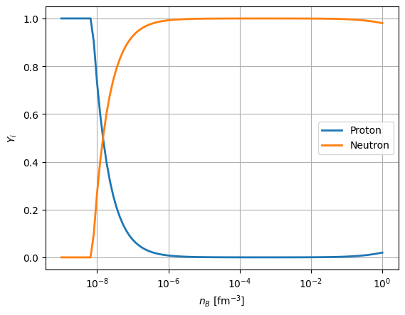
To check that the tables have been correctly created, we can use the Interface class as described in Section Creating interpolated tables, to run the CompOSE code. In this quick example, we create an interpolated table for the proton and neutron mass fractions.
[25]:
from compytools import (
    GridSettings,
    Interface,
    summarise
)
[26]:
# Show available particle mass fractions
summarise(tmpdir.name, tables='compo')
            Available particle mass fractions.
┏━━━━━━━━━━━━━━━━━┳━━━━━━━━━━━━━━━┳━━━━━━━━━━━━━━━━┳━━━━━━┓
┃ Quantity Number ┃ Quantity Name ┃ Quantity Index ┃ Unit ┃
┡━━━━━━━━━━━━━━━━━╇━━━━━━━━━━━━━━━╇━━━━━━━━━━━━━━━━╇━━━━━━┩
│ 1               │ electron      │ 0              │      │
│ 2               │ proton        │ 11             │      │
│ 3               │ neutron       │ 10             │      │
└─────────────────┴───────────────┴────────────────┴──────┘
     Nuclear particle indices.
┏━━━━━━━━━━━━━━━━━┳━━━━━━━━━━━━━━━━┓
┃ Quantity number ┃ Particle index ┃
┡━━━━━━━━━━━━━━━━━╇━━━━━━━━━━━━━━━━┩
│ 1               │ 1              │
└─────────────────┴────────────────┘
[27]:
nbconfig = GridSettings(
    min=1.e-10,
    max=1.0,
    order=1,
    npoints=100,
    logscale=True
)

interface = Interface(
    eospath=tmpdir.name,
    # Choose proton and neutron mass fractions
    particle_choice=[2, 3],
    nbconfig=nbconfig
)

table = interface.run()
table.pprint()
INFO File /tmp/tmp9y1phlfh/eos.table created. interface.py:682
    T          nb         Yq     Y (proton) Y (neutron)
   MeV      1 / fm3
---------- ---------- ---------- ---------- -----------
0.0000e+00 1.0001e-09 0.0000e+00 1.0000e+00  0.0000e+00
0.0000e+00 1.2330e-09 0.0000e+00 1.0000e+00  0.0000e+00
0.0000e+00 1.5201e-09 0.0000e+00 1.0000e+00  0.0000e+00
0.0000e+00 1.8740e-09 0.0000e+00 1.0000e+00  0.0000e+00
0.0000e+00 2.3104e-09 0.0000e+00 1.0000e+00  0.0000e+00
0.0000e+00 2.8483e-09 0.0000e+00 1.0000e+00  0.0000e+00
0.0000e+00 3.5115e-09 0.0000e+00 1.0000e+00  0.0000e+00
0.0000e+00 4.3292e-09 0.0000e+00 1.0000e+00  0.0000e+00
0.0000e+00 5.3372e-09 0.0000e+00 1.0000e+00  0.0000e+00
       ...        ...        ...        ...         ...
0.0000e+00 1.5199e-01 0.0000e+00 4.6869e-03  9.9531e-01
0.0000e+00 1.8738e-01 0.0000e+00 5.5826e-03  9.9442e-01
0.0000e+00 2.3101e-01 0.0000e+00 6.6349e-03  9.9337e-01
0.0000e+00 2.8481e-01 0.0000e+00 7.8644e-03  9.9214e-01
0.0000e+00 3.5112e-01 0.0000e+00 9.2925e-03  9.9071e-01
0.0000e+00 4.3288e-01 0.0000e+00 1.0935e-02  9.8907e-01
0.0000e+00 5.3367e-01 0.0000e+00 1.2811e-02  9.8719e-01
0.0000e+00 6.5793e-01 0.0000e+00 1.4940e-02  9.8506e-01
0.0000e+00 8.1113e-01 0.0000e+00 1.7335e-02  9.8267e-01
0.0000e+00 1.0000e+00 0.0000e+00 2.0004e-02  9.8000e-01
Length = 100 rows
[28]:
plt.figure()
plt.semilogx(table['nb'], table['Y (proton)'], linewidth=2, label='Proton')
plt.semilogx(table['nb'], table['Y (neutron)'], linewidth=2, label='Neutron')

plt.legend()
plt.grid()

plt.xlabel(r'$n_{B}$ [fm$^{-3}$]')
plt.ylabel(r'$Y_{i}$')
[28]:
Text(0, 0.5, '$Y_{i}$')