Reading CompOSE tables
In this section, we demonstrate how ComPyTools can be used to:
read equation of state (EoS) tables in the
CompOSEformat,inspect the data and associated metadata,
extract a subset of the data needed for a given analysis, with some corresponding examples.
[1]:
import os
import tempfile

from compytools.download import CompOSEDownloader

# For the purposes of this documentation create a
# temporary directory into which to download a sample
# set of tables for the demonstration
tmpdir = tempfile.TemporaryDirectory()

# Download some sample data to work with
# PCP(BSk22): https://compose.obspm.fr/eos/256
downloader = CompOSEDownloader.from_eosname('PCP(BSk22)', tmpdir.name)
downloader.get()
[2]:
os.listdir(tmpdir.name)
[2]:
['README',
 'eos.micro',
 'eos.t',
 'eos.thermo',
 'eos.yq',
 'eos.pdf',
 'eos.init',
 'eos.zip',
 'eos.nb',
 'eos.compo',
 'eos.mr']
The files that are relevant for us here are the following:
eos.thermo: contains the thermodynamic quantities,eos.[t,nb,yq]: contains the grid parameters for temperaturet, baryon number densitynband charge fractionyq,eos.compo: holds the composition (particle number fractions and nuclear data),eos.mr: contains the neutron star static properties (mass and radius, for example) calculated with this EoS.
These table can be read with the following command, specifying the directory containing the tables:
[3]:
from compytools import EoS

bsk22 = EoS.from_compose(tmpdir.name)
ComPyTools performs quality checks on the data, notably:
Whether data contains invalid values such as NaNs or infinities,
Monotonicity checks on pressure, enthalpy per baryon (cold tables only),
Monotonicity checks on the grid parameters,
Acausality and instability checks on the sound speed,
Whether the entropy per baryon and lepton chemical potential are zero (cold tables only).
Data associated with a given table can be accessed with the following dot . notation. For example, to view the data associated with the eos.compo file:
[4]:
# Use the pprint to "pretty print" the table to screen.
# the wax_width=-1 option prints the entire width of the table to screen.
bsk22.compo.pprint(max_width=-1)
 iT jnB kYq Iphase Npairs    Y_0        Y_1        Y_10       Y_11    Nquads Inuc_1   Aav_1      Zav_1      Ynuc_1

--- --- --- ------ ------ ---------- ---------- ---------- ---------- ------ ------ ---------- ---------- ----------
  0   1   1      1      4 4.6429e-01 0.0000e+00 0.0000e+00 0.0000e+00      1      1 5.6000e+01 2.6000e+01 1.0000e+00
  0   2   1      1      4 4.6429e-01 0.0000e+00 0.0000e+00 0.0000e+00      1      1 5.6000e+01 2.6000e+01 1.0000e+00
  0   3   1      1      4 4.6429e-01 0.0000e+00 0.0000e+00 0.0000e+00      1      1 5.6000e+01 2.6000e+01 1.0000e+00
  0   4   1      1      4 4.6429e-01 0.0000e+00 0.0000e+00 0.0000e+00      1      1 5.6000e+01 2.6000e+01 1.0000e+00
  0   5   1      1      4 4.6429e-01 0.0000e+00 0.0000e+00 0.0000e+00      1      1 5.6000e+01 2.6000e+01 1.0000e+00
  0   6   1      1      4 4.6429e-01 0.0000e+00 0.0000e+00 0.0000e+00      1      1 5.6000e+01 2.6000e+01 1.0000e+00
  0   7   1      1      4 4.6429e-01 0.0000e+00 0.0000e+00 0.0000e+00      1      1 5.6000e+01 2.6000e+01 1.0000e+00
  0   8   1      1      4 4.6429e-01 0.0000e+00 0.0000e+00 0.0000e+00      1      1 5.6000e+01 2.6000e+01 1.0000e+00
  0   9   1      1      4 4.6429e-01 0.0000e+00 0.0000e+00 0.0000e+00      1      1 5.6000e+01 2.6000e+01 1.0000e+00
... ... ...    ...    ...        ...        ...        ...        ...    ...    ...        ...        ...        ...
  0 480   1      0      4 2.2346e-01 2.0223e-01 5.7432e-01 4.2568e-01      1      1 0.0000e+00 0.0000e+00 0.0000e+00
  0 481   1      0      4 2.2385e-01 2.0271e-01 5.7344e-01 4.2656e-01      1      1 0.0000e+00 0.0000e+00 0.0000e+00
  0 482   1      0      4 2.2424e-01 2.0319e-01 5.7257e-01 4.2743e-01      1      1 0.0000e+00 0.0000e+00 0.0000e+00
  0 483   1      0      4 2.2463e-01 2.0365e-01 5.7172e-01 4.2828e-01      1      1 0.0000e+00 0.0000e+00 0.0000e+00
  0 484   1      0      4 2.2500e-01 2.0411e-01 5.7089e-01 4.2911e-01      1      1 0.0000e+00 0.0000e+00 0.0000e+00
  0 485   1      0      4 2.2537e-01 2.0456e-01 5.7007e-01 4.2993e-01      1      1 0.0000e+00 0.0000e+00 0.0000e+00
  0 486   1      0      4 2.2573e-01 2.0501e-01 5.6926e-01 4.3074e-01      1      1 0.0000e+00 0.0000e+00 0.0000e+00
  0 487   1      0      4 2.2609e-01 2.0545e-01 5.6847e-01 4.3153e-01      1      1 0.0000e+00 0.0000e+00 0.0000e+00
  0 488   1      0      4 2.2644e-01 2.0588e-01 5.6769e-01 4.3231e-01      1      1 0.0000e+00 0.0000e+00 0.0000e+00
  0 489   1      0      4 2.2678e-01 2.0630e-01 5.6692e-01 4.3308e-01      1      1 0.0000e+00 0.0000e+00 0.0000e+00
Length = 489 rows
which shows not only column headers, but also units for each column (where applicable). Additional descriptions for each column can be accessed via the info method:
[5]:
bsk22.compo.info
[5]:
<Compo length=489>
 name   dtype  format                    description                     class
------ ------- ------ ------------------------------------------------- --------
    iT   int32     %d                            Temperature grid point   Column
   jnB   int32     %d                    Baryon num. density grid point   Column
   kYq   int32     %d                   Charge num. fraction grid point   Column
Iphase   int32     %d               indexing encoding the type of phase   Column
Npairs   int32     %d Num. of paired particle, num. fraction quantities   Column
   Y_0 float32   %.4e               Num. fraction for particle electron Quantity
   Y_1 float32   %.4e                   Num. fraction for particle muon Quantity
  Y_10 float32   %.4e                Num. fraction for particle neutron Quantity
  Y_11 float32   %.4e                 Num. fraction for particle proton Quantity
Nquads   int32     %d             Num. of quadrupled nuclear quantities   Column
Inuc_1   int32     %d                 Particle index for particle set 1   Column
 Aav_1 float32   %.4e   Av. mass num. of representative nucleus (set 1) Quantity
 Zav_1 float32   %.4e Av. charge num. of representative nucleus (set 1) Quantity
Ynuc_1 float32   %.4e Combined nuclear num. fraction for particle set 1 Quantity
Data for a given column, for example the number fraction of electrons, Y_0, can be accessed via
[6]:
bsk22.compo['Y_0']
[6]:
Data for the eos.thermo, eos.mr and eos.micro tables can similarly be accessed with bsk22.thermo, bsk22.mr and bsk22.micro, respectively.
Finally, grid points can be displayed with:
[7]:
bsk22.params
[7]:
Grid(t=<Param length=1>
    t
   MeV
 float32
----------
0.0000e+00, nb=<Param length=489>
    nb
 1 / fm3
 float32
----------
4.6796e-10
5.8496e-10
7.3385e-10
9.2229e-10
1.1613e-09
1.4652e-09
1.8525e-09
2.3471e-09
2.9801e-09
       ...
1.4122e+00
1.4222e+00
1.4322e+00
1.4422e+00
1.4522e+00
1.4622e+00
1.4722e+00
1.4822e+00
1.4922e+00, yq=<Param length=1>
    yq

 float32
----------
0.0000e+00)
and individual grid points, for example for the baryon number density nb, can be accessed with:
[8]:
bsk22.params.nb.grid_points
[8]:
Grid points for temperature and charge fraction can similarly accessed with bsk22.params.t.grid_points and bsk22.params.yq.grid_points.
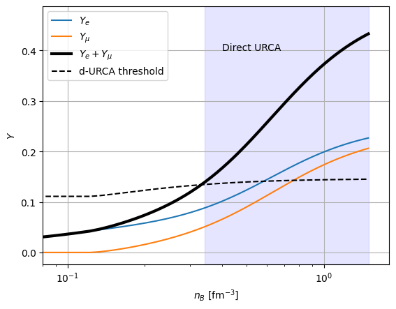
Example 1: Calculating the direct URCA threshold
Here, we demonstrate how the aforementioned functionality can be used to calculate and plot the threshold for the direct URCA process for our sample EoS.
See Section 3.10 in https://compose.obspm.fr/manual/ for further details.
[9]:
import numpy as np
import matplotlib.pyplot as plt


def Yq_direct_URCA(Ye, Ymu):
    """
    Calculate the criterion in the charge fraction at which
    the direct URCA process is expected to take place.

    Parameters
    ----------
    Ye
        Electron fraction [adim]
    Ymu
        Muon fraction [adim]

    """
    ratio = Ye / (Ye + Ymu)
    term1 = np.pow(ratio, 1/3)
    term2 = np.pow(1 + term1, 3)

    return 1 / (1 + term2)
[10]:
# This module defines useful constants and units
from compytools.constants import PERFM3

YdURCA = Yq_direct_URCA(bsk22.compo['Y_0'], bsk22.compo['Y_1'])

# Fractions for electrons and muons
Ye = bsk22.compo['Y_0']
Ymu = bsk22.compo['Y_1']

# Total charge fraction
Yq = Ye + Ymu

# Get the baryon number density grid points
# and the crust-core boundary
nb = bsk22.params.nb.grid_points

# Assign units to the baryon num. density at core-crust transition.
# This is needed if we wish to work with the baryon num. density
# which has units assigned to them.
nb_cc = 0.08 << PERFM3

nb_dURCA = nb[Yq >= YdURCA]
# Limit the range of the baryon number density to the core region
nb_dURCA = np.min(nb_dURCA[nb_dURCA >= nb_cc])
[11]:
plt.plot(nb, Ye, label=r'$Y_{e}$')
plt.plot(nb, Ymu, label=r'$Y_{\mu}$')
plt.plot(nb, Yq, '-k', linewidth=3, label=r'$Y_{e}+Y_{\mu}$')
plt.plot(nb, YdURCA, '--k', label='d-URCA threshold')

plt.axvspan(nb_dURCA.value, 1.5, color='blue', alpha=0.1)

plt.xscale('log')
plt.grid()
plt.legend()

plt.xlabel(r'$n_{B}$ [fm$^{-3}$]')
plt.ylabel(r'$Y$')
plt.text(0.4, 0.4, 'Direct URCA')
plt.xlim(0.08, 1.8)
plt.show()
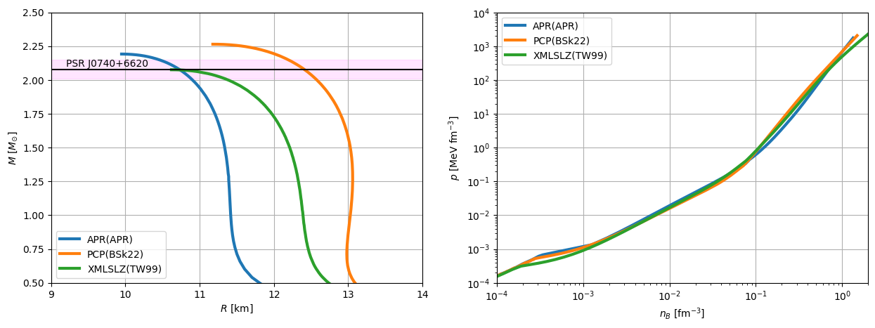
Example 2: Comparing mass-radius and pressure-baryon number density curves for several EoSs
The OOP design means that it is straightforward to compare data between several EoSs.
[12]:
EOS_LIST = [
    # APR(APR) from https://compose.obspm.fr/eos/68
    'APR(APR)',
    # PCP(BSk22): https://compose.obspm.fr/eos/256
    'PCP(BSk22)',
    # XMLSLZ(TW99) from https://compose.obspm.fr/eos/288
    'XMLSLZ(TW99)'
]

eos = {}
for eos_name in EOS_LIST:
    # Download each eos into its own (temporary) directory
    tmpdir = tempfile.TemporaryDirectory()
    getter = CompOSEDownloader.from_eosname(eos_name, tmpdir.name)
    getter.get()

    # Store each EoS instance into a dictionary. Turn off the checks
    # to keep the output cleaner.
    eos[eos_name] = EoS.from_compose(tmpdir.name, do_checks=False)
[13]:
plt.figure(figsize=(15, 5))
plt.subplot(121)
# Compare the mass-radius curves against the mass of the pulsar PSR J0740+6620
for name in list(eos.keys()):
    plt.plot(eos[name].mr['radius'], eos[name].mr['mass'], linewidth=3, label=name)

plt.text(9.2, 2.1 ,'PSR J0740+6620')
plt.axhspan(2.01, 2.15, color='magenta', alpha=0.1)
plt.axhline(2.08, color='k')
plt.grid()
plt.legend()

plt.xlim(9., 14)
plt.ylim(0.5, 2.5)
plt.xlabel(r'$R$ [km]')
plt.ylabel(r'$M$ [$M_{\odot}$]')

plt.subplot(122)
# Compare the pressures as a function of the baryon number density
# for each equation of state.
for name in list(eos.keys()):
    nb = eos[name].params.nb.grid_points
    pressure = nb * eos[name].thermo['Q1']

    plt.loglog(nb, pressure, label=name, linewidth=3)

plt.grid()
plt.legend()

plt.xlim(1.e-4, 2.0)
plt.ylim(1.e-4, 1.e4)

plt.xlabel(r'$n_B$ [fm$^{-3}$]')
plt.ylabel(r'$p$ [MeV fm$^{-3}$]')
[13]:
Text(0, 0.5, '$p$ [MeV fm$^{-3}$]')
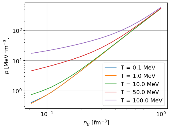
Example 3: General purpose tables - impact of temperature on pressure
ComPyTools can also read general purpose tables. Here we demonstrate how data “slices” can be extracted in order to investigate how the temperature affects pressure in the core region of the neutron star.
[14]:
# Download a sample data into a temporary directory
tmpdir = tempfile.TemporaryDirectory()

# RG(SLy4): https://compose.obspm.fr/eos/148
getter = CompOSEDownloader.from_eosname('RG(SLy4)', tmpdir.name)
getter.get()
General purpose tables can be read using multiple cores via the ncores argument to the from_compose method:
[15]:
sly4 = EoS.from_compose(tmpdir.name, ncores=4)
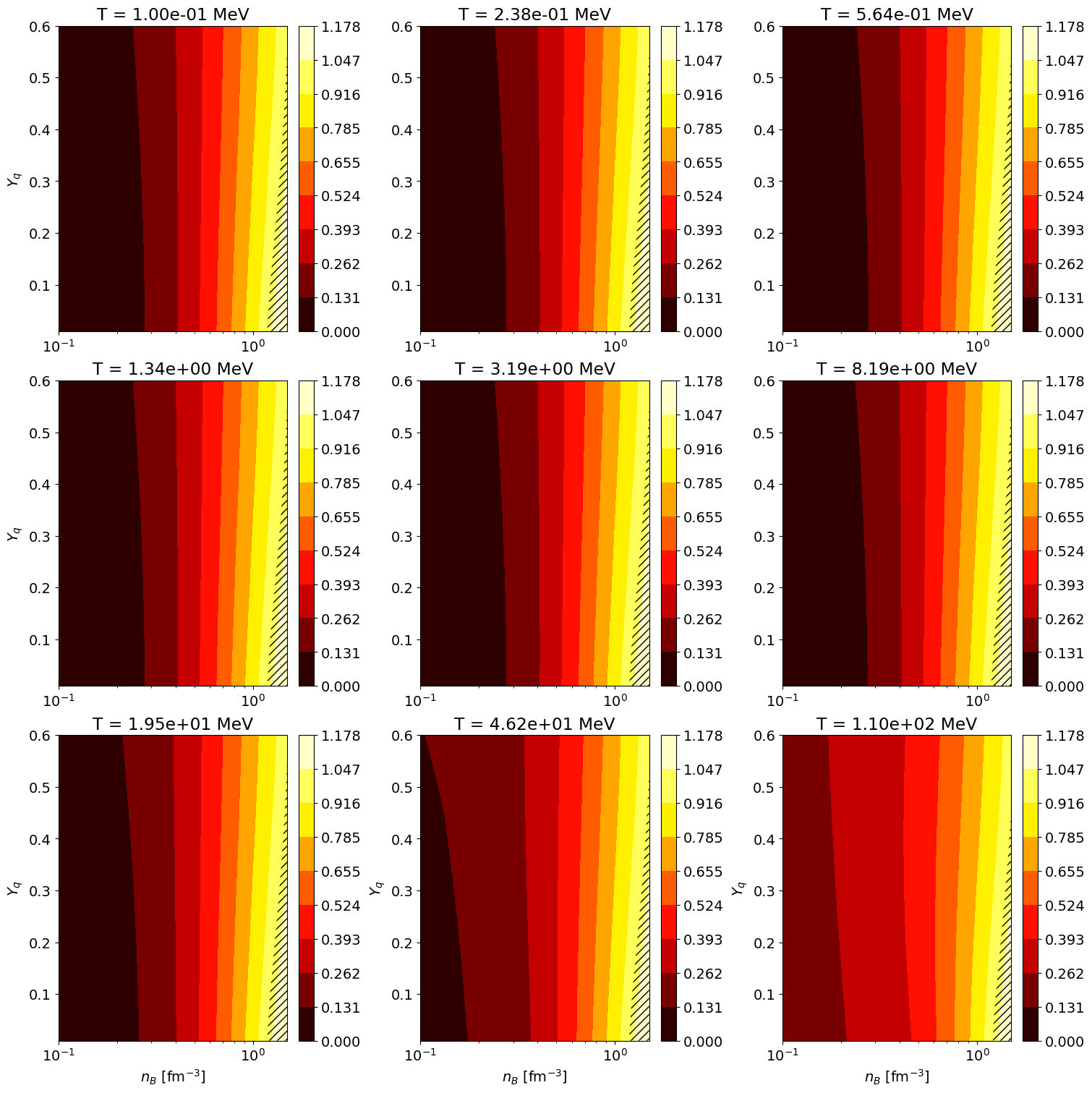
As part of the quality control checks, a figure is produced and saved to a file called cs2.png which is located in the same directory as the EoS tables. The figure shows the square of the sound speed, \(c_{s}^{2}\), as a function of the baryon number density, \(n_{B}\), and the charge number fraction, \(Y_{q}\), for several slices in temperature, \(T\). Acausal regions are indicated by hatched regions.
In this example, we will examine the pressure versus baryon number density for several values of temperature \(T=(0.1, 1.0, 10.0, 50, 100)\) MeV for a fixed charge fraction of \(Y_{q}=0.01\). We will also consider baryon number densities corresponding to the core region \(0.08\leq{n_{B}}/\mathrm{fm}^{-3}\leq{1}\).
We use the select method to filter out data for the specifies ranges in baryon number density nBrange, charge fraction Yqrange and temperature Trange.
The select method can also be similarly applied for the compo and micro data tables.
[16]:
temperatures = [
    0.1,
    1.,
    10.,
    50.,
    100.
]

for temp in temperatures:
    table = sly4.thermo.select(
        # Ranges in baryon number density, charge fraction
        # and temperature
        nBrange=(0.08, 1.0),
        Yqrange=(0.01, 0.01),
        Trange=(temp, temp),
        # Variables we wish to extract. Here, the ratio between
        # pressure and baryon number density
        vars=['Q1'],
        # EoS grid parameters
        grid_params=sly4.params
    )

    # The resulting table will automatically contain the grid points
    # in temperature, 't', baryon number density 'nb and charge fraction
    # 'yq'.
    pressure = table['Q1'] * table['nb']
    plt.loglog(table['nb'], pressure, label=f'T = {temp} MeV')
    plt.grid()
    plt.legend()

    plt.xlabel(r'$n_{B}$ [fm$^{-3}$]')
    plt.ylabel(r'$p$ [MeV fm$^{-3}$]')