Creating tables in the CompOSE format II - Mandatory and optional tables
This section describes how a contributor can provide the mandatory files (i.e. the grid parameter files eos.t, eos.nb and eos.yq and the table holding the thermodynamic quantities eos.thermo) as well as the optional files (eos.compo, eos.micro and eos.mr) that hold the composition, microphysics and the static neutron star properties, respectively. We consider a cold equation of state (EoS) in the CompOSE format.
Functionality to write general purpose tables will be provided in a future release of ComPyTools.
We then describe how to create the PDF data sheet that summarises the information about the EoS. This is a document that exists along side the aforementioned tables on the CompOSE web-site and provides human-readable information concerning the EoS.
In this example, we illustrate how to produce the aforementioned CompOSE files using raw data associated with the PCP(BSk24) EoS. This example may be particularly useful since it also highlights how to combine data contained in separate files. However, to keep the example simple yet illustrative, we will just produce the EoS associated to the inner crust and the core only.
We will consider the following files:
eos_BSk24.dat: This contains the EoS for the core and has the following quantities:
Column number |
Quantity |
unit |
|---|---|---|
1 |
Baryon num. density |
fm\(^{-3}\) |
2 |
Energy density |
MeV fm\(^{-3}\) |
3 |
Pressure |
MeV fm\(^{-3}\) |
4 |
Electron num. fraction |
|
5 |
Muon num. fraction |
|
6 |
Neutron chemical potential |
MeV |
7 |
Proton chemical potential |
MeV |
8 |
Electron chemical potential |
MeV |
9 |
Muon chemical potential |
MeV |
10 |
Neutron effective mass divided by neutron bare mass |
|
11 |
Proton effective mass divided by neutron bare mass |
|
12 |
Neutron non-relativistic single-particle potential |
MeV |
13 |
Proton non-relativistic single-particle potential |
MeV |
eq24.dat: This contains the EoS for the inner crust and consists of the following quantities:
Column number |
Quantity |
unit |
|---|---|---|
1 |
Baryon num. density |
fm\(^{-3}\) |
2 |
Proton number in Wigner-Seitz cell |
|
3 |
Proton number fraction |
|
4 |
Neutron number in Wigner-Seitz cell |
|
5 |
Mass number in Wigner-Seitz cell |
|
8 |
Pressure |
MeV fm\(^{-3}\) |
10 |
Energy per baryon\(^{*}\) |
MeV |
15 |
Proton chemical potential\(^{*}\) |
MeV |
16 |
Neutron chemical potential\(^{*}\) |
MeV |
17 |
Electron chemical potential\(^{*}\) |
MeV |
26 |
Proton number |
|
27 |
Neutron number |
|
28 |
Mass number |
The asterisked quantities indicate that the neutron rest mass energy is not taken into account.
GapNeutronCore_BSk24.dat and GapProtonCore_BSk24.dat: The second column of these files contain the neutron and proton gap energies in the core.
These files were kindly provided by Nicolas Chamel and Anthea F. Fantina. For further information about the PCP(BSk24) EoS, the interested reader is referred to Pearson et al. 2018: https://doi.org/10.1093/mnras/sty2413) and Pearson et al. 2019: https://doi.org/10.1093/mnras/stz800.
Let’s download the data and load it.
For the purposes of this tutorial, to avoid polluting the file system with output files, we output the CompOSE tables into a temporary directory. However, if you are following along and you wish to keep the files, you can replace tmpdir.name with the directory path of your choice.
[1]:
import os
import tempfile
import requests
import warnings
warnings.filterwarnings("ignore", "Wswiglal-redir-stdio")

import numpy as np

tmpdir = tempfile.TemporaryDirectory()
files = [
    "eos_BSk24.dat",
    "eq24.dat",
    "GapNeutronCore_BSk24.dat",
    "GapProtonCore_BSk24.dat",
]

eos_url = "https://gitlab.in2p3.fr/lpc-caen/compytools/-/raw/main/tests/inputs/PCP(BSk24)/"

for _file in files:
    source = os.path.join(eos_url, _file)
    dest = os.path.join(tmpdir.name, _file)

    response = requests.get(source)
    with open(dest, 'wb') as context:
        context.write(response.content)
[2]:
# Load the EoS for the inner crust
(
    nb_crust,
    Zws_crust,
    Yp_crust,
    Nws_crust,
    Aws_crust,
    p_crust,
    e_crust,
    mup_crust,
    mun_crust,
    mue_crust,
    Z_crust,
    N_crust,
    A_crust
) = np.loadtxt(
    os.path.join(tmpdir.name, 'eq24.dat'),
    usecols=(0, 1, 2, 3, 4, 7, 9, 14, 15, 16, 25, 26, 27),
    unpack=True
)

# Load the EoS data for the core
(
    nb_core,
    eps_core,
    p_core,
    Ye_core,
    Ymu_core,
    mun_core,
    mup_core,
    mue_core,
    mumu_core,
    meffn_core,
    meffp_core,
    Un_core,
    Up_core
) = np.loadtxt(os.path.join(tmpdir.name, 'eos_BSk24.dat'), unpack=True)
ComPyTools provides a set of user-friendly interfaces that allows the contributor to provide the required information in order to create the necessary tables. These interfaces allow the user to carry out the following steps:
Feed the data into a data structure and provide units. This allows the code to perform sanity checking on the units, perform conversions if necessary and compute automatically any additional quantities expected by
CompOSE,This data structure is then coverted into a tabulated form, allowing the user to view and inspect the data. This tabular form also makes it possible to write the data to file further down the line.
The procedure is described below for each of the tables in turn.
Grid parameter files (eos.[t,nb,yq])
Store the grid points into a data structure via the GridData class. For cold tables there is only a single value for temperature and charge fraction, which are both zero:
[3]:
from compytools import (
    GridData,
    Grid
)

from compytools.constants import (
    DIMENSIONLESS,
    MEV,
    PERFM3
)

# Concatenate the crust and the core grid points together
nb = np.concatenate((nb_crust, nb_core))

grid_data = GridData(
    t=np.array([0.0]) << MEV,
    nb=nb << PERFM3,
    yq=np.array([0.0]) << DIMENSIONLESS
)

grid_params = Grid.from_dataset(grid_data)
Here and elsewhere, it is mandatory to provide units even if they are already in the units as required by CompOSE. This not only allows ComPyTools to perform sanity checking on the input data, but it also allows units to be added to the table’s metadata.
Here and elsewhere, we use the syntax << (or alternatively *) to provide units for each provided quantity. Next, create tables for each of the grid parameters using the Grid class.
[4]:
grid_params = Grid.from_dataset(grid_data)
We can access the grid points for the baryon number. Note how the units are attached to the data array.
[5]:
grid_params.nb.grid_points
[5]:
The syntax to access grid points for temperature t and charge fraction yq is similar.
Thermodynamics (eos.thermo)
A similar procedure as described above the grid parameter data is followed for the remaining tables.
Here we provide the data for the eos.thermo table.
[6]:
from compytools import (
    ExtraThermoQuantity,
    Nucleons,
    ThermoData,
    Thermo
)

from compytools.constants import (
    MEV_PER_FM3
)
The header information that specifies the neutron and proton masses, and the flag indicating whether leptons are included, is provided via the Nucleons class:
[7]:
mn = 939.5651828
mp = 938.271844
nucleons = Nucleons(
    mn=mn << MEV,
    mp=mp << MEV,
    has_leptons=1
)
print(nucleons)
Nucleons(has_leptons=1, mn=<Quantity 939.5651828 MeV>, mp=<Quantity 938.271844 MeV>)
Now we need to concatenate together thermodynamic quantities associated with the crust and with the core:
[8]:
# Combined electron chemical potential
mue = np.concatenate((mue_crust, mue_core)) << MEV

# Charge chemical potential
muq = -mue

# Calculate the energy density in the crust, including the rest-mass energy and
# combine with the core energy density
eps_crust = (e_crust + mn) * nb_crust
energy_density = np.concatenate((eps_crust, eps_core)) << MEV_PER_FM3

# Add the rest-mass energy to the neutron chemical potential in the crust and
# combine with that in the core
mun_crust += mn
mun = np.concatenate((mun_crust, mun_core)) << MEV

# Combine the pressure in crust and core
press = np.concatenate((p_crust, p_core)) << MEV_PER_FM3
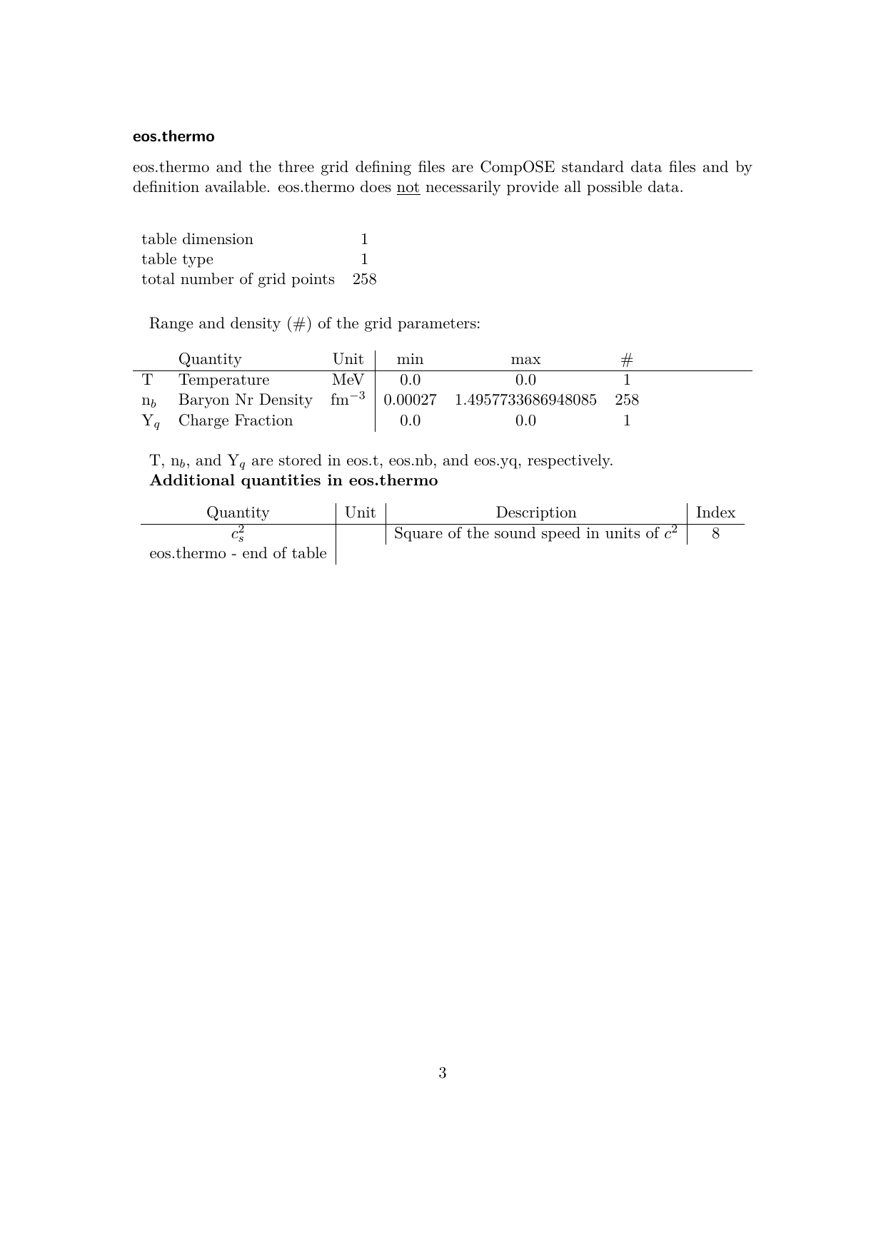
We will also demonstrate how to provide an additional thermodynamic quantity by providing the square of the speed of sound, \(c_{s}^{2}\) which will be in units of the square of the speed of light, \(c\). Since we take \(c=1\), \(c_{s}^{2}\) will be dimensionless.
[9]:
cs2 = np.gradient(press, energy_density)
Note that, in this example, the pressure and the energy density are already in the required units needed in order to calculate \(c_{s}^{2}\). If this is not the case, then astropy provides functionality that allows the user to easily convert units. For example, if pressure are provided in dyn cm\(^{-2}\) and energy density in g cm\(^{-2}\), then we can convert into MeV fm\(^{-3}\) using the following:
import astropy.units as u

from compytools import DYN_PER_CM2, G_PER_CM3, MEV_PER_FM3

total_pressure = (p << DYN_PER_CM2).to(MEV_PER_FM3)
rho = rho << G_PER_CM3

energy_density = rho.to(MEV_PER_FM3, equivalencies=u.mass_energy())
cs2 = np.gradient(total_pressure, energy_density, edge_order=2)
Also note that the equivalencies=u.mass_energy() argument allows us to convert units into relativistic units. For further information, the interested user is referred to the astropy documentation.
Additional quantities are provided via a dictionary:
The key of the dictionary gives the variable name. You can use \(\LaTeX\) syntax which will allow the variable name to be correctly displayed within the PDF data sheet,
The value of the key is a class
ExtraThermoQuantitywhere you provide the array, units and a description. The latter will be used to create the appropriate entry in the data sheet.
[10]:
extra_thermo = {
    '$c_{s}^{2}$': ExtraThermoQuantity(
        data=cs2,
        unit=DIMENSIONLESS,
        description='Square of the sound speed in units of $c^2$')
}
Now, let’s create the thermodynamic data structure and then the Thermo table:
[11]:
thermo_data = ThermoData(
    grid_params=grid_params,
    nucleons=nucleons,
    pressure=press,
    # The entropy is zero for cold matter
    entropy_density=np.zeros(nb.size) << PERFM3,
    baryon_chemical_potential=mun,
    charge_chemical_potential=muq,
    # Lepton chemical potential is zero for a cold table
    lepton_chemical_potential=np.zeros(nb.size) << MEV,
    free_energy_density=energy_density,
    internal_energy_density=energy_density,
    # Additional quantities can be provided via the Qextra argument
    Qextra=extra_thermo
)

thermo = Thermo.from_dataset(thermo_data)
Note that, since the units for the pressure, neutron chemical potential, charge chemical potential and energy density were specified already above, they don’t need to be specified again in the ThermoData class.
Also note that if the baryon chemical potential, \(\mu_{\mathrm{B}}\), is not known, the baryon_chemical_potential argument above can be omitted, in which case it will be automatically calculated via
for the case of a cold EoS. Here, \(p\) is the pressure, \(e\) is the internal energy density and \(n_{\mathrm{B}}\) is the baryon number density.
As per the CompOSE convention, the rest mass should be included in the chemical potentials.
The data, as well as the associated metadata (i.e. descriptions of each of the columns and their units), can be accessed with the respective methods:
[12]:
# The max_width argument allows you to provide the maximum number of characters to display in the table.
# Set a value of -1 to impose no limit.
thermo.pprint(max_width=-1)
thermo.info
 iT jnB kYq     Q1         Q2         Q3          Q4         Q5          Q6          Q7     Nextra $c_{s}^{2}$
               MeV
--- --- --- ---------- ---------- ---------- ----------- ---------- ----------- ----------- ------ -----------
  0   1   1 1.9042e+00 0.0000e+00 1.8574e-04 -2.7863e-02 0.0000e+00 -1.8410e-03 -1.8410e-03      1  1.0417e-03
  0   2   1 1.8014e+00 0.0000e+00 2.9540e-04 -2.8276e-02 0.0000e+00 -1.6219e-03 -1.6219e-03      1  9.7800e-04
  0   3   1 1.6959e+00 0.0000e+00 3.8962e-04 -2.8638e-02 0.0000e+00 -1.4154e-03 -1.4154e-03      1  8.8900e-04
  0   4   1 1.5983e+00 0.0000e+00 4.8024e-04 -2.8988e-02 0.0000e+00 -1.2208e-03 -1.2208e-03      1  8.6703e-04
  0   5   1 1.5109e+00 0.0000e+00 5.7099e-04 -2.9338e-02 0.0000e+00 -1.0371e-03 -1.0371e-03      1  8.7021e-04
  0   6   1 1.4347e+00 0.0000e+00 6.6395e-04 -2.9696e-02 0.0000e+00 -8.6298e-04 -8.6298e-04      1  8.8774e-04
  0   7   1 1.3693e+00 0.0000e+00 7.6032e-04 -3.0066e-02 0.0000e+00 -6.9702e-04 -6.9702e-04      1  9.1455e-04
  0   8   1 1.3144e+00 0.0000e+00 8.6098e-04 -3.0452e-02 0.0000e+00 -5.3795e-04 -5.3795e-04      1  9.4875e-04
  0   9   1 1.2696e+00 0.0000e+00 9.6667e-04 -3.0857e-02 0.0000e+00 -3.8455e-04 -3.8455e-04      1  9.8887e-04
... ... ...        ...        ...        ...         ...        ...         ...         ...    ...         ...
  0 249   1 1.2566e+03 0.0000e+00 2.0927e+00 -4.3717e-01 0.0000e+00  7.5526e-01  7.5526e-01      1  1.1818e+00
  0 250   1 1.2721e+03 0.0000e+00 2.1188e+00 -4.3856e-01 0.0000e+00  7.6480e-01  7.6480e-01      1  1.1867e+00
  0 251   1 1.2878e+03 0.0000e+00 2.1450e+00 -4.3994e-01 0.0000e+00  7.7439e-01  7.7439e-01      1  1.1916e+00
  0 252   1 1.3035e+03 0.0000e+00 2.1713e+00 -4.4131e-01 0.0000e+00  7.8403e-01  7.8403e-01      1  1.1964e+00
  0 253   1 1.3193e+03 0.0000e+00 2.1978e+00 -4.4267e-01 0.0000e+00  7.9371e-01  7.9371e-01      1  1.2011e+00
  0 254   1 1.3351e+03 0.0000e+00 2.2245e+00 -4.4401e-01 0.0000e+00  8.0345e-01  8.0345e-01      1  1.2058e+00
  0 255   1 1.3511e+03 0.0000e+00 2.2513e+00 -4.4535e-01 0.0000e+00  8.1324e-01  8.1324e-01      1  1.2105e+00
  0 256   1 1.3672e+03 0.0000e+00 2.2782e+00 -4.4668e-01 0.0000e+00  8.2307e-01  8.2307e-01      1  1.2151e+00
  0 257   1 1.3833e+03 0.0000e+00 2.3052e+00 -4.4800e-01 0.0000e+00  8.3296e-01  8.3296e-01      1  1.2196e+00
  0 258   1 1.3995e+03 0.0000e+00 2.3324e+00 -4.4931e-01 0.0000e+00  8.4289e-01  8.4289e-01      1  1.2219e+00
Length = 258 rows
[12]:
<Thermo length=258>
    name     dtype  unit format                    description                      class
----------- ------- ---- ------ -------------------------------------------------- --------
         iT   int32          %d                             Temperature grid point   Column
        jnB   int32          %d                     Baryon num. density grid point   Column
        kYq   int32          %d                    Charge num. fraction grid point   Column
         Q1 float32  MeV   %.4e       pressure divided by baryon num. density p/nb Quantity
         Q2 float32        %.4e                            entropy per baryon s/nb Quantity
         Q3 float32        %.4e scaled and shifted baryon chem. potential mub/mn-1 Quantity
         Q4 float32        %.4e            scaled charge chemical potential muq/mn Quantity
         Q5 float32        %.4e  scaled effective lepton chemical potential mul/mn Quantity
         Q6 float32        %.4e      scaled free energy per baryon f/(nb x mn) - 1 Quantity
         Q7 float32        %.4e  scaled internal energy per baryon e/(nb x mn) - 1 Quantity
     Nextra   int32          %d                num. extra thermodynamic quantities   Column
$c_{s}^{2}$ float32        %.4e        Square of the sound speed in units of $c^2$ Quantity
If you are using this functionality in your scripts you will need to use Python’s print() function, i.e. print(thermo.pprint(max_width=-1)) and print(thermo.info).
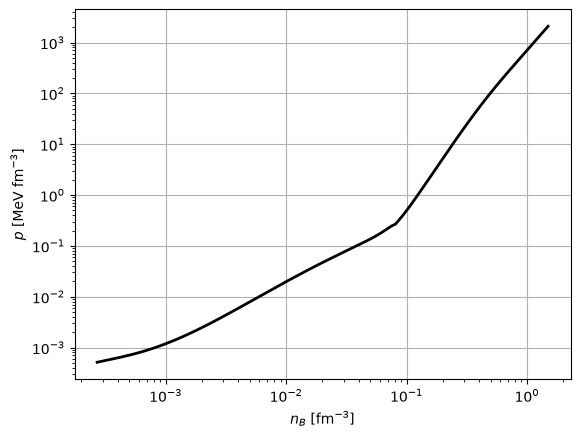
Data can be accessed (for example for plotting) as described in the Section Reading CompOSE tables. For example, to access the data associated with the ratio of the pressure and the baryon number density \(p/n_{\mathrm{B}}\), we can use the syntax thermo['Q1']:
[13]:
import matplotlib.pyplot as plt

plt.figure()

nb = grid_params.nb.grid_points
pressure = nb * thermo['Q1']
plt.loglog(nb, pressure, '-k', linewidth=2)

plt.xlabel(r'$n_{B}$ [fm$^{-3}$]')
plt.ylabel(r'$p$ [MeV fm$^{-3}$]')
plt.grid()
Composition (eos.compo)
[14]:
from compytools import (
    Compo,
    CompoData,
    NuclearSet
)
First, lets give the number fractions for each of the particles that are considered by PCP(BSk24). We use a Python dictionary to provide these fractions, where the key for each entry has the form Y (<particle_name>) and <particle_name> should be replaced by the name of the particle. The list of available particle names considered by CompOSE is displayed by running the following function:
[15]:
from compytools import show_particles

show_particles()
           Available CompOSE particles.
┏━━━━━━━━━━━━━━━━┳━━━━━━━━━━━━━━━┳━━━━━━━━━━━━━━━┓
┃ Particle Index ┃ Particle Name ┃ Particle type ┃
┡━━━━━━━━━━━━━━━━╇━━━━━━━━━━━━━━━╇━━━━━━━━━━━━━━━┩
│ 0              │ electron      │ lepton        │
│ 1              │ muon          │ lepton        │
│ 10             │ neutron       │ baryon        │
│ 11             │ proton        │ baryon        │
│ 20             │ Delta^-       │ baryon        │
│ 21             │ Delta^0       │ baryon        │
│ 22             │ Delta^+       │ baryon        │
│ 23             │ Delta^++      │ baryon        │
│ 100            │ Lambda        │ baryon        │
│ 110            │ Sigma^-       │ baryon        │
│ 111            │ Sigma^0       │ baryon        │
│ 112            │ Sigma^+       │ baryon        │
│ 120            │ Xi^-          │ baryon        │
│ 121            │ Xi^0          │ baryon        │
│ 200            │ omega         │ meson         │
│ 210            │ sigma         │ meson         │
│ 220            │ eta           │ meson         │
│ 230            │ eta^prime     │ meson         │
│ 300            │ rho^-         │ meson         │
│ 301            │ rho^0         │ meson         │
│ 302            │ rho^+         │ meson         │
│ 310            │ delta^-       │ meson         │
│ 311            │ delta^0       │ meson         │
│ 312            │ delta^+       │ meson         │
│ 320            │ pi^-          │ meson         │
│ 321            │ pi^0          │ meson         │
│ 322            │ pi^+          │ meson         │
│ 400            │ phi           │ meson         │
│ 410            │ sigma_s       │ meson         │
│ 420            │ K^-           │ meson         │
│ 421            │ K^0           │ meson         │
│ 422            │ Kbar^0        │ meson         │
│ 423            │ K^+           │ meson         │
│ 500            │ u quark       │ quark         │
│ 501            │ d quark       │ quark         │
│ 502            │ s quark       │ quark         │
│ 600            │ photon        │ photon        │
│ 2001           │ deuteron 2H   │ nuclei        │
│ 3001           │ triton 3H     │ nuclei        │
│ 3002           │ helion 3He    │ nuclei        │
│ 4002           │ alpha 4He     │ nuclei        │
└────────────────┴───────────────┴───────────────┘
This table corresponds to Tables 3.3, 3.4 and 3.5 in the CompOSE manual https://compose.obspm.fr/manual.
[16]:
# Electron and proton number fractions in crust equal due to charge neutrality
Ye_crust = Yp_crust
Ye = np.concatenate((Ye_crust, Ye_core)) << DIMENSIONLESS

# Calculate free protons in the crust and core
Ypfree_crust = (Zws_crust-Z_crust)/Aws_crust
# Charge neutrality
Ypfree_core = Ye_core + Ymu_core
Ypfree = np.concatenate((Ypfree_crust, Ypfree_core)) << DIMENSIONLESS

# Calculate the free neutrons in the crust and core
Ynfree_crust = (Nws_crust-N_crust)/Aws_crust
Ynfree_core = 1 - Ypfree_core
Ynfree = np.concatenate((Ynfree_crust, Ynfree_core)) << DIMENSIONLESS

# Number fraction of muons
# There are no muons in the crust
Ymu_crust = np.zeros(nb_crust.size)
Ymu = np.concatenate((Ymu_crust, Ymu_core)) << DIMENSIONLESS

particle_fractions = {
    'Y (electron)': Ye,
    'Y (proton)': Ypfree,
    'Y (neutron)': Ynfree,
    'Y (muon)': Ymu
}
Note that a space needs to be provided between “Y” and the particle name, as per the formatting rules for the dictionary keys in particle_fractions.
We can also provide, for an index \(I_{i}\) that specifies a group of nuclei \(\mathcal{M}_{I_{i}}\), an average mass number Aav, proton number Zav and combined fraction Ynuc via the NuclearSet interface as follows:
[17]:
# Mass number. Note that this is zero in the core since there are no nuclei here
A_core = np.zeros(nb_core.size)
Aav = np.concatenate((A_crust, A_core)) << DIMENSIONLESS

# Proton number. Note that this is zero in the core
Z_core = np.zeros(nb_core.size)
Zav = np.concatenate((Z_crust, Z_core)) << DIMENSIONLESS

# Calculate the number fraction of nuclei
# ... from the conservation of baryon number
Ynuc_crust = (1 - Ypfree_crust - Ynfree_crust) / A_crust
# No Nuclei in the core
Ynuc_core = np.zeros(nb_core.size)
Ynuc = np.concatenate((Ynuc_crust, Ynuc_core)) << DIMENSIONLESS

nuclear_sets = {
    1: NuclearSet(
        Aav=Aav,
        Zav=Zav,
        Ynuc=Ynuc
    )
}
Alternatively, if no nuclear sets are to be provided by the user, one can specify nuclear_sets=None.
Here, the dictionary key gives the value \(I_{i}\) for a given nuclear set.
Next, provide the phase indices that define the neutron star structure. For PCP(BSk24), we follow the convention of the original authors and use an index 0 to indicate homogenous matter in the core, while index 2 indicates the inner crust. The core region is located where the baryon number density is larger than the baryon number density at the crust-core interface:
[18]:
# Grab the first grid point in the core region.
# Since nb possesses a unit, we must also provide a unit for nb_cc
# so that units are consistent in the inequality.
nb_cc = nb_core[0] * PERFM3
Iphase = np.where(nb>=nb_cc, 0, 2)
Now provide the data via the CompoData interface and then create the data table with the Compo class:
[19]:
compo_data = CompoData(
    grid_params=grid_params,
    Iphase=Iphase,
    particle_fractions=particle_fractions,
    nuclear_sets=nuclear_sets
)

compo = Compo.from_dataset(compo_data)
compo.pprint(max_width=125)
compo.info
 iT jnB kYq Iphase Npairs Y (electron) Y (proton) ...  Y (muon)  Nquads Inuc (set #1) Aav (set #1) Zav (set #1) Ynuc (set #1)
                                                  ...
--- --- --- ------ ------ ------------ ---------- ... ---------- ------ ------------- ------------ ------------ -------------
  0   1   1      2      4   2.9091e-01 8.7274e-06 ... 0.0000e+00      1             1   1.3232e+02   3.9999e+01    7.2729e-03
  0   2   1      2      4   2.7027e-01 8.1079e-06 ... 0.0000e+00      1             1   1.3316e+02   3.9999e+01    6.7566e-03
  0   3   1      2      4   2.4958e-01 7.4873e-06 ... 0.0000e+00      1             1   1.3389e+02   3.9999e+01    6.2394e-03
  0   4   1      2      4   2.3008e-01 6.9023e-06 ... 0.0000e+00      1             1   1.3459e+02   3.9999e+01    5.7519e-03
  0   5   1      2      4   2.1202e-01 6.3605e-06 ... 0.0000e+00      1             1   1.3529e+02   3.9999e+01    5.3004e-03
  0   6   1      2      4   1.9545e-01 5.8634e-06 ... 0.0000e+00      1             1   1.3601e+02   3.9999e+01    4.8862e-03
  0   7   1      2      4   1.8031e-01 5.4094e-06 ... 0.0000e+00      1             1   1.3675e+02   3.9999e+01    4.5078e-03
  0   8   1      2      4   1.6654e-01 5.4124e-06 ... 0.0000e+00      1             1   1.3752e+02   3.9999e+01    4.1634e-03
  0   9   1      2      4   1.5402e-01 5.0056e-06 ... 0.0000e+00      1             1   1.3832e+02   3.9999e+01    3.8505e-03
... ... ...    ...    ...          ...        ... ...        ...    ...           ...          ...          ...           ...
  0 249   1      0      4   2.1594e-01 4.1094e-01 ... 1.9499e-01      1             1   0.0000e+00   0.0000e+00    0.0000e+00
  0 250   1      0      4   2.1647e-01 4.1206e-01 ... 1.9560e-01      1             1   0.0000e+00   0.0000e+00    0.0000e+00
  0 251   1      0      4   2.1698e-01 4.1317e-01 ... 1.9619e-01      1             1   0.0000e+00   0.0000e+00    0.0000e+00
  0 252   1      0      4   2.1748e-01 4.1426e-01 ... 1.9678e-01      1             1   0.0000e+00   0.0000e+00    0.0000e+00
  0 253   1      0      4   2.1798e-01 4.1533e-01 ... 1.9735e-01      1             1   0.0000e+00   0.0000e+00    0.0000e+00
  0 254   1      0      4   2.1847e-01 4.1638e-01 ... 1.9791e-01      1             1   0.0000e+00   0.0000e+00    0.0000e+00
  0 255   1      0      4   2.1894e-01 4.1741e-01 ... 1.9847e-01      1             1   0.0000e+00   0.0000e+00    0.0000e+00
  0 256   1      0      4   2.1941e-01 4.1842e-01 ... 1.9901e-01      1             1   0.0000e+00   0.0000e+00    0.0000e+00
  0 257   1      0      4   2.1987e-01 4.1942e-01 ... 1.9955e-01      1             1   0.0000e+00   0.0000e+00    0.0000e+00
  0 258   1      0      4   2.2032e-01 4.2040e-01 ... 2.0007e-01      1             1   0.0000e+00   0.0000e+00    0.0000e+00
Length = 258 rows
[19]:
<Compo length=258>
     name      dtype  format                    description                        class
------------- ------- ------ ------------------------------------------------- --------------
           iT   int32      d                            Temperature grid point         Column
          jnB   int32      d                    Baryon num. density grid point         Column
          kYq   int32      d                   Charge num. fraction grid point         Column
       Iphase   int32      d               indexing encoding the type of phase         Column
       Npairs   int32      d Num. of paired particle, num. fraction quantities         Column
 Y (electron) float32    .4e               Num. fraction for particle electron MaskedQuantity
   Y (proton) float32    .4e                 Num. fraction for particle proton MaskedQuantity
  Y (neutron) float32    .4e                Num. fraction for particle neutron MaskedQuantity
     Y (muon) float32    .4e                   Num. fraction for particle muon MaskedQuantity
       Nquads   int32      d             Num. of quadrupled nuclear quantities         Column
Inuc (set #1)   int32      d                 Particle index for particle set 1   MaskedColumn
 Aav (set #1) float32    .4e   Av. mass num. of representative nucleus (set 1) MaskedQuantity
 Zav (set #1) float32    .4e Av. charge num. of representative nucleus (set 1) MaskedQuantity
Ynuc (set #1) float32    .4e Combined nuclear num. fraction for particle set 1 MaskedQuantity
Microphysics (eos.micro)
The microphysics quantities are provided via a dictionary where the keys take the form <quantity> (<particle_name>). The available particle names can be listed using the aforementioned function show_particles(), while the list of available microphysics quantities can be shown with:
[20]:
from compytools import show_microphysics

show_microphysics()
                                    Available CompOSE microphysics quantities.
┏━━━━━━━━━━━━━━━━━━━━┳━━━━━━━━━━━━━━━━━━━━━━━━━┳━━━━━━━━━━━━━━━━━━━━━━━━━━━━━━━━━━━━━━━━━━━━━━━━━━━━━━━━━━━┳━━━━━━┓
┃ Microphysics Index ┃ Microphysics Quantity   ┃ Description                                               ┃ Unit ┃
┡━━━━━━━━━━━━━━━━━━━━╇━━━━━━━━━━━━━━━━━━━━━━━━━╇━━━━━━━━━━━━━━━━━━━━━━━━━━━━━━━━━━━━━━━━━━━━━━━━━━━━━━━━━━━╇━━━━━━┩
│ 40                 │ m_L/m (<particle_name>) │ Landau effective mass divided by particle mass            │      │
│                    │                         │ $m_{i}^{L}/m_{i}$ (<particle_name>)                       │      │
│ 41                 │ m_D/m (<particle_name>) │ Dirac effective mass divided by particle mass             │      │
│                    │                         │ $m_{i}^{D}/m_{i}$ (<particle_name>)                       │      │
│ 50                 │ U (<particle_name>)     │ Non-relativistic single particle potential $U_{i}$        │ MeV  │
│                    │                         │ (<particle_name>)                                         │      │
│ 51                 │ V (<particle_name>)     │ Relativistic vector self-energy $V_{i}$ (<particle_name>) │ MeV  │
│ 52                 │ S (<particle_name>)     │ Relativistic scalar self-energy $S_{i}$ (<particle_name>) │ MeV  │
│ 60                 │ Delta (<particle_name>) │ Pairing gap in the (<particle_name>) channel              │ MeV  │
└────────────────────┴─────────────────────────┴───────────────────────────────────────────────────────────┴──────┘
This table corresponds to Table 7.5 in the CompOSE manual https://compose.obspm.fr/manual.
Here, we will provide:
Landau effective mass divided by the bare mass (for protons and neutrons),
Non-relativistic particle potential (protons and neutrons),
Pairing gap energy for neutron-neutron and proton-proton correlations.
Concerning the pairing gap, this only applies to two-particle correlations. To view the available correlations, once can use the show_particle_correlations() function:
[21]:
from compytools import show_particle_correlations

show_particle_correlations()
     Available CompOSE two-particle
             correlations.
┏━━━━━━━━━━━━━━━━━━━┳━━━━━━━━━━━━━━━━━━┓
┃ Correlation index ┃ Correlation Name ┃
┡━━━━━━━━━━━━━━━━━━━╇━━━━━━━━━━━━━━━━━━┩
│ 700               │ nn (1S0)         │
│ 701               │ np (1S0)         │
│ 702               │ pp (1S0)         │
│ 703               │ np (3S1)         │
└───────────────────┴──────────────────┘
[22]:
# Set the ratio of the effective mass to bare mass to 1 in
# the crust
meffn_crust = np.full(nb_crust.size, 1)
meffp_crust = np.full(nb_crust.size, 1)
meffn = np.concatenate((meffn_crust, meffn_core)) << DIMENSIONLESS
meffp = np.concatenate((meffp_crust, meffp_core)) << DIMENSIONLESS

# Set the single particle potential to zero in the crust
Un_crust = np.zeros(nb_crust.size)
Up_crust = np.zeros(nb_crust.size)
Un = np.concatenate((Un_crust, Un_core)) << MEV
Up = np.concatenate((Up_crust, Up_core)) << MEV

# Set the gap energy to zero in the crust, and load the core values
# from file.
Deltap_crust = np.zeros(nb_crust.size)
Deltan_crust = np.zeros(nb_crust.size)
Deltap_core = np.loadtxt(
    os.path.join(tmpdir.name, 'GapProtonCore_BSk24.dat'),
    usecols=(1,)
)
Deltan_core = np.loadtxt(
    os.path.join(tmpdir.name,'GapNeutronCore_BSk24.dat'),
    usecols=(1,)
)

Deltap = np.concatenate((Deltan_crust, Deltan_core)) << MEV
Deltan = np.concatenate((Deltap_crust, Deltap_core)) << MEV

microphysics = {
    'm_L/m (neutron)': meffn,
    'm_L/m (proton)': meffp,
    'U (neutron)': Un,
    'U (proton)': Up,
    'Delta (nn (1S0))': Deltan,
    'Delta (pp (1S0))': Deltap
}
Now let’s feed in the information into the MicroData and Micro classes:
[23]:
from compytools import (
    Micro,
    MicroData
)

micro_data = MicroData(
    grid_params=grid_params,
    microphysics=microphysics
)

micro = Micro.from_dataset(micro_data)
micro.pprint(max_width=-1)
micro.info
 iT jnB kYq Npairs m_L/m (neutron) m_L/m (proton) U (neutron) U (proton) Delta (nn (1S0)) Delta (pp (1S0))
                                                      MeV        MeV           MeV              MeV
--- --- --- ------ --------------- -------------- ----------- ---------- ---------------- ----------------
  0   1   1      6      1.0000e+00     1.0000e+00  0.0000e+00 0.0000e+00       0.0000e+00       0.0000e+00
  0   2   1      6      1.0000e+00     1.0000e+00  0.0000e+00 0.0000e+00       0.0000e+00       0.0000e+00
  0   3   1      6      1.0000e+00     1.0000e+00  0.0000e+00 0.0000e+00       0.0000e+00       0.0000e+00
  0   4   1      6      1.0000e+00     1.0000e+00  0.0000e+00 0.0000e+00       0.0000e+00       0.0000e+00
  0   5   1      6      1.0000e+00     1.0000e+00  0.0000e+00 0.0000e+00       0.0000e+00       0.0000e+00
  0   6   1      6      1.0000e+00     1.0000e+00  0.0000e+00 0.0000e+00       0.0000e+00       0.0000e+00
  0   7   1      6      1.0000e+00     1.0000e+00  0.0000e+00 0.0000e+00       0.0000e+00       0.0000e+00
  0   8   1      6      1.0000e+00     1.0000e+00  0.0000e+00 0.0000e+00       0.0000e+00       0.0000e+00
  0   9   1      6      1.0000e+00     1.0000e+00  0.0000e+00 0.0000e+00       0.0000e+00       0.0000e+00
... ... ...    ...             ...            ...         ...        ...              ...              ...
  0 249   1      6      1.4409e-01     1.6650e-01  7.5252e+02 7.9181e+02       0.0000e+00       0.0000e+00
  0 250   1      6      1.4308e-01     1.6518e-01  7.6420e+02 8.0423e+02       0.0000e+00       0.0000e+00
  0 251   1      6      1.4208e-01     1.6387e-01  7.7594e+02 8.1670e+02       0.0000e+00       0.0000e+00
  0 252   1      6      1.4109e-01     1.6258e-01  7.8776e+02 8.2923e+02       0.0000e+00       0.0000e+00
  0 253   1      6      1.4012e-01     1.6130e-01  7.9965e+02 8.4182e+02       0.0000e+00       0.0000e+00
  0 254   1      6      1.3916e-01     1.6005e-01  8.1160e+02 8.5447e+02       0.0000e+00       0.0000e+00
  0 255   1      6      1.3821e-01     1.5881e-01  8.2362e+02 8.6718e+02       0.0000e+00       0.0000e+00
  0 256   1      6      1.3727e-01     1.5759e-01  8.3571e+02 8.7994e+02       0.0000e+00       0.0000e+00
  0 257   1      6      1.3635e-01     1.5639e-01  8.4787e+02 8.9276e+02       0.0000e+00       0.0000e+00
  0 258   1      6      1.3543e-01     1.5520e-01  8.6010e+02 9.0563e+02       0.0000e+00       0.0000e+00
Length = 258 rows
[23]:
<Micro length=258>
      name        dtype  unit format                                description                                     class
---------------- ------- ---- ------ -------------------------------------------------------------------------- --------------
              iT   int32           d                                                     Temperature grid point         Column
             jnB   int32           d                                             Baryon num. density grid point         Column
             kYq   int32           d                                            Charge num. fraction grid point         Column
          Npairs   int32           d                                                  Num. of paired quantities         Column
 m_L/m (neutron) float32         .4e Landau effective mass divided by particle mass $m_{i}^{L}/m_{i}$ (neutron) MaskedQuantity
  m_L/m (proton) float32         .4e  Landau effective mass divided by particle mass $m_{i}^{L}/m_{i}$ (proton) MaskedQuantity
     U (neutron) float32  MeV    .4e               Non-relativistic single particle potential $U_{i}$ (neutron) MaskedQuantity
      U (proton) float32  MeV    .4e                Non-relativistic single particle potential $U_{i}$ (proton) MaskedQuantity
Delta (nn (1S0)) float32  MeV    .4e                                      Pairing gap in the (nn (1S0)) channel MaskedQuantity
Delta (pp (1S0)) float32  MeV    .4e                                      Pairing gap in the (pp (1S0)) channel MaskedQuantity
Note that the user may have the values of the Landau masses or the Dirac masses instead of the ratios m_L/m or m_D/m for a given particle. To calculate the ratios that are required by the micro table, the mass for the desired particle (if this is not already known by the user) can be accessed using the function get_particle_mass. For example, to get the mass of the Lambda hyperon:
[24]:
from compytools import get_particle_mass

ml = get_particle_mass('Lambda')
print(ml)
1115.683138712051 MeV
where the unit is automatically attached to the mass. Thus, if one has an array of effective masses, one can proceed as follows as illustrated in this simple example:
[25]:
# A mock data set containing the effective masses of the Lambda hyperon, with the units attached
meff_lambda = [1115.68, 1115.68, 1000.0, 800.0] << MEV
meff_lambda_over_ml = meff_lambda / ml

print(meff_lambda_over_ml)
[0.99999719 0.99999719 0.89631183 0.71704947]
The list of available baryons/ hyperon names (which can be used an an argument to the get_particle_mass function) and their masses, can be accessed with the show_baryon_masses function:
[26]:
from compytools import show_baryon_masses

show_baryon_masses()
    Available CompOSE baryon/ hyperon masses.
┏━━━━━━━━━━━━━━━━┳━━━━━━━━━━━━━━━┳━━━━━━━━━━━━━━━┓
┃ Particle Index ┃ Particle Name ┃ Particle Mass ┃
┡━━━━━━━━━━━━━━━━╇━━━━━━━━━━━━━━━╇━━━━━━━━━━━━━━━┩
│ 10             │ neutron       │ 939.565 MeV   │
│ 11             │ proton        │ 938.272 MeV   │
│ 20             │ Delta^-       │ 1232.000 MeV  │
│ 21             │ Delta^0       │ 1232.000 MeV  │
│ 22             │ Delta^+       │ 1232.000 MeV  │
│ 23             │ Delta^++      │ 1232.000 MeV  │
│ 100            │ Lambda        │ 1115.683 MeV  │
│ 110            │ Sigma^-       │ 1197.449 MeV  │
│ 111            │ Sigma^0       │ 1192.642 MeV  │
│ 112            │ Sigma^+       │ 1189.370 MeV  │
│ 120            │ Xi^-          │ 1321.711 MeV  │
│ 121            │ Xi^0          │ 1314.861 MeV  │
└────────────────┴───────────────┴───────────────┘
We use the 2025 values of the particle masses as provided by the Particle Data Group (PDG). For masses of the deuterion, triton, helion and the alpha particle, we use the CODATA 2022 values.
Instead of using the PDG particle values, you can also choose to use your own values.
Neutron star properties
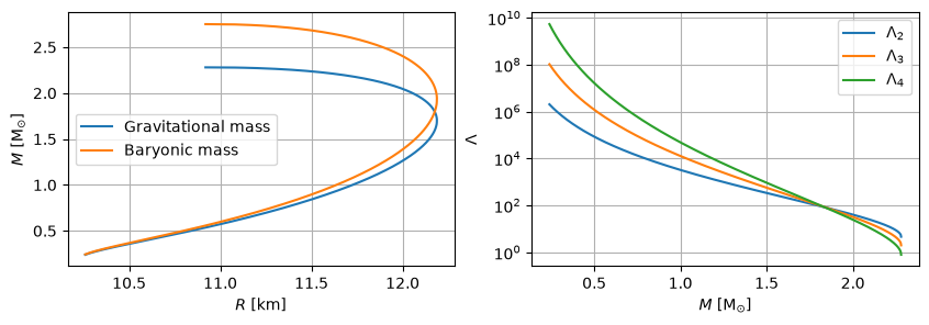
ComPyTools includes the lalsimulation package that is part of the lalsuite library. The lalsimulation package includes a solver for the Tolman-Oppenheimer-Volkoff equations that allows the user to automatically calculate several static neutron star properties based on the input EoS. The quantities are:
The radius in km,
The gravitational mass in solar masses,
The quadrupole tidal deformability (adim, multipole order \(\ell=2\)),
The central baryon number density in fm\(^{-3}\),
The baryonic mass in solar masses,
The octupole tidal deformability (adim, \(\ell=3\)),
The hexadecapole tidal deformability (adim, \(\ell=4\)).
These quantities are calculated via the NeutronStarData class by supplying the grid parameters, the thermodynamical table and (if it is available) the table containing the composition.
[27]:
from compytools import (
    NeutronStar,
    NeutronStarData,
)

ns_data = NeutronStarData(
    grid_params=grid_params,
    thermo=thermo,
    compo=compo
)

mr = NeutronStar.from_dataset(ns_data)
mr.pprint(max_width=-1)
mr.info
  radius   mass_grav   Lambda2   central_baryon_num_density mass_baryonic  Lambda3    Lambda4
    km      solMass                       1 / fm3              solMass
---------- ---------- ---------- -------------------------- ------------- ---------- ----------
1.0259e+01 2.4018e-01 2.0539e+06                 1.8451e-01    2.4418e-01 1.0562e+08 5.4244e+09
1.0262e+01 2.4222e-01 1.9808e+06                 1.8508e-01    2.4630e-01 1.0032e+08 5.0683e+09
1.0265e+01 2.4426e-01 1.9109e+06                 1.8565e-01    2.4842e-01 9.5329e+07 4.7381e+09
1.0268e+01 2.4631e-01 1.8440e+06                 1.8621e-01    2.5054e-01 9.0627e+07 4.4321e+09
1.0270e+01 2.4835e-01 1.7801e+06                 1.8676e-01    2.5266e-01 8.6194e+07 4.1485e+09
1.0273e+01 2.5039e-01 1.7189e+06                 1.8732e-01    2.5477e-01 8.2014e+07 3.8857e+09
1.0276e+01 2.5243e-01 1.6602e+06                 1.8787e-01    2.5689e-01 7.8068e+07 3.6424e+09
1.0279e+01 2.5447e-01 1.6040e+06                 1.8842e-01    2.5901e-01 7.4343e+07 3.4171e+09
1.0283e+01 2.5651e-01 1.5501e+06                 1.8896e-01    2.6114e-01 7.0825e+07 3.2081e+09
       ...        ...        ...                        ...           ...        ...        ...
1.1323e+01 2.2617e+00 7.6053e+00                 8.5384e-01    2.7216e+00 3.6754e+00 1.6610e+00
1.1302e+01 2.2637e+00 7.3930e+00                 8.6049e-01    2.7248e+00 3.5470e+00 1.5904e+00
1.1281e+01 2.2658e+00 7.1779e+00                 8.6747e-01    2.7280e+00 3.4180e+00 1.5200e+00
1.1258e+01 2.2678e+00 6.9544e+00                 8.7513e-01    2.7312e+00 3.2853e+00 1.4482e+00
1.1232e+01 2.2698e+00 6.7188e+00                 8.8368e-01    2.7345e+00 3.1469e+00 1.3741e+00
1.1204e+01 2.2719e+00 6.4740e+00                 8.9300e-01    2.7377e+00 3.0045e+00 1.2987e+00
1.1170e+01 2.2739e+00 6.2039e+00                 9.0413e-01    2.7409e+00 2.8494e+00 1.2176e+00
1.1131e+01 2.2760e+00 5.9088e+00                 9.1709e-01    2.7441e+00 2.6823e+00 1.1313e+00
1.1081e+01 2.2780e+00 5.5580e+00                 9.3393e-01    2.7474e+00 2.4869e+00 1.0320e+00
1.0919e+01 2.2800e+00 4.6366e+00                 9.8905e-01    2.7507e+00 1.9918e+00 7.8905e-01
Length = 1000 rows
[27]:
<NeutronStar length=1000>
           name             dtype    unit  format           description             class
-------------------------- ------- ------- ------ -------------------------------- --------
                    radius float64      km   %.4e              Neutron star radius Quantity
                 mass_grav float64 solMass   %.4e  Neutron star gravitational mass Quantity
                   Lambda2 float64           %.4e   Quadrupole tidal deformability Quantity
central_baryon_num_density float64 1 / fm3   %.4e    Central baryon number density Quantity
             mass_baryonic float64 solMass   %.4e       Neutron star baryonic mass Quantity
                   Lambda3 float64           %.4e     Octupole tidal deformability Quantity
                   Lambda4 float64           %.4e Hexadecapole tidal deformability Quantity
Note that if the composition is not available for the equation of state, then the compo argument in NeutronStarData can be omitted.
Let’s plot the data:
[28]:
plt.figure(figsize=(10, 3))
plt.subplot(121)
plt.plot(mr['radius'], mr['mass_grav'], label='Gravitational mass')
plt.plot(mr['radius'], mr['mass_baryonic'], label='Baryonic mass')
plt.legend()
plt.grid()
plt.xlabel(r'$R$ [km]')
plt.ylabel(r'$M$ [M$_{\odot}$]')

plt.subplot(122)
plt.semilogy(mr['mass_grav'], mr['Lambda2'], label=r'$\Lambda_{2}$')
plt.semilogy(mr['mass_grav'], mr['Lambda3'], label=r'$\Lambda_{3}$')
plt.semilogy(mr['mass_grav'], mr['Lambda4'], label=r'$\Lambda_{4}$')
plt.legend()
plt.grid()
plt.xlabel(r'$M$ [M$_{\odot}]$')
plt.ylabel(r'$\Lambda$')
[28]:
Text(0, 0.5, '$\\Lambda$')
Writing the CompOSE tables
Once we have created a data table associated to each of the CompOSE tables, we now combine them together using the EoS class. This allows ComPyTools to perform quality checks:
Whether the data contains invalid values such as NaNs, infinities or values that are not floats,
Sound speed checks (acausality and negative values),
Monotonicity checks on pressure and enthalpy, as well as for the grid point values,
Whether the entropy and lepton chemical potentials are indeed zero for cold tables,
Whether the baryon number fraction is conserved.
[29]:
import tempfile

from compytools import EoS

# For the purposes of this tutorial create a temporary directory into which
# to write the tables.
tmpdir = tempfile.TemporaryDirectory()

eos = EoS(
    params=grid_params,
    thermo=thermo,
    compo=compo,
    micro=micro,
    mr=mr
)
[30]:
eos.to_compose(tmpdir.name)

# List the contents of the directory
os.listdir(tmpdir.name)
[30]:
['eos.micro',
 'eos.t',
 'eos.thermo',
 'eos.yq',
 'eos.init',
 'eos.nb',
 'eos.compo',
 'eos.mr']
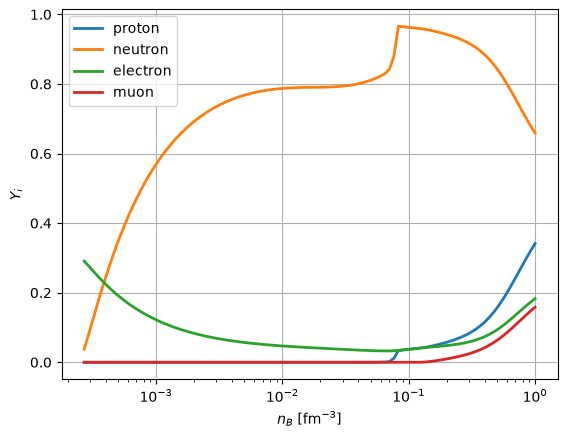
To check that the tables have been correctly created, we can use the Interface class as described in Section Creating interpolated tables, to run the CompOSE code. In this quick example, we create an interpolated table for the proton and neutron mass fractions.
[31]:
from compytools import (
    GridSettings,
    Interface,
    summarise
)
[32]:
# Show available particle mass fractions
summarise(tmpdir.name, tables='compo')
            Available particle mass fractions.
┏━━━━━━━━━━━━━━━━━┳━━━━━━━━━━━━━━━┳━━━━━━━━━━━━━━━━┳━━━━━━┓
┃ Quantity Number ┃ Quantity Name ┃ Quantity Index ┃ Unit ┃
┡━━━━━━━━━━━━━━━━━╇━━━━━━━━━━━━━━━╇━━━━━━━━━━━━━━━━╇━━━━━━┩
│ 1               │ electron      │ 0              │      │
│ 2               │ proton        │ 11             │      │
│ 3               │ neutron       │ 10             │      │
│ 4               │ muon          │ 1              │      │
└─────────────────┴───────────────┴────────────────┴──────┘
     Nuclear particle indices.
┏━━━━━━━━━━━━━━━━━┳━━━━━━━━━━━━━━━━┓
┃ Quantity number ┃ Particle index ┃
┡━━━━━━━━━━━━━━━━━╇━━━━━━━━━━━━━━━━┩
│ 1               │ 1              │
└─────────────────┴────────────────┘
[33]:
nbconfig = GridSettings(
    min=1.e-10,
    max=1.0,
    order=1,
    npoints=100,
    logscale=True
)

interface = Interface(
    eospath=tmpdir.name,
    # Choose proton and neutron mass fractions
    particle_choice=[1, 2, 3, 4],
    nbconfig=nbconfig
)

table = interface.run()
table.pprint()
INFO File /tmp/tmpog8img1n/eos.table created. interface.py:682
    T          nb         Yq     Y (electron) Y (proton) Y (neutron)  Y (muon)
   MeV      1 / fm3
---------- ---------- ---------- ------------ ---------- ----------- ----------
0.0000e+00 2.7003e-04 0.0000e+00   2.9090e-01 8.7269e-06  3.7680e-02 0.0000e+00
0.0000e+00 2.9340e-04 0.0000e+00   2.7660e-01 8.2980e-06  8.1050e-02 0.0000e+00
0.0000e+00 3.1879e-04 0.0000e+00   2.6207e-01 7.8622e-06  1.2574e-01 0.0000e+00
0.0000e+00 3.4637e-04 0.0000e+00   2.4745e-01 7.4236e-06  1.7126e-01 0.0000e+00
0.0000e+00 3.7635e-04 0.0000e+00   2.3377e-01 7.0130e-06  2.1424e-01 0.0000e+00
0.0000e+00 4.0892e-04 0.0000e+00   2.2087e-01 6.6262e-06  2.5490e-01 0.0000e+00
0.0000e+00 4.4431e-04 0.0000e+00   2.0839e-01 6.2518e-06  2.9438e-01 0.0000e+00
0.0000e+00 4.8276e-04 0.0000e+00   1.9661e-01 5.8982e-06  3.3175e-01 0.0000e+00
0.0000e+00 5.2454e-04 0.0000e+00   1.8599e-01 5.5798e-06  3.6549e-01 0.0000e+00
       ...        ...        ...          ...        ...         ...        ...
0.0000e+00 4.7379e-01 0.0000e+00   8.7823e-02 1.4511e-01  8.5489e-01 5.7283e-02
0.0000e+00 5.1479e-01 0.0000e+00   9.6309e-02 1.6259e-01  8.3741e-01 6.6279e-02
0.0000e+00 5.5934e-01 0.0000e+00   1.0581e-01 1.8210e-01  8.1790e-01 7.6290e-02
0.0000e+00 6.0775e-01 0.0000e+00   1.1620e-01 2.0341e-01  7.9659e-01 8.7213e-02
0.0000e+00 6.6034e-01 0.0000e+00   1.2728e-01 2.2613e-01  7.7387e-01 9.8858e-02
0.0000e+00 7.1749e-01 0.0000e+00   1.3877e-01 2.4974e-01  7.5026e-01 1.1097e-01
0.0000e+00 7.7958e-01 0.0000e+00   1.5036e-01 2.7362e-01  7.2638e-01 1.2325e-01
0.0000e+00 8.4705e-01 0.0000e+00   1.6177e-01 2.9718e-01  7.0282e-01 1.3541e-01
0.0000e+00 9.2035e-01 0.0000e+00   1.7271e-01 3.1986e-01  6.8014e-01 1.4715e-01
0.0000e+00 1.0000e+00 0.0000e+00   1.8298e-01 3.4125e-01  6.5875e-01 1.5827e-01
Length = 100 rows
[34]:
plt.figure()

particles = [
    'proton',
    'neutron',
    'electron',
    'muon'
]

for particle in particles:
    plt.semilogx(table['nb'], table[f'Y ({particle})'], linewidth=2, label=f'{particle}')

plt.legend()
plt.grid()

plt.xlabel(r'$n_{B}$ [fm$^{-3}$]')
plt.ylabel(r'$Y_{i}$')
[34]:
Text(0, 0.5, '$Y_{i}$')
Creating the data sheet
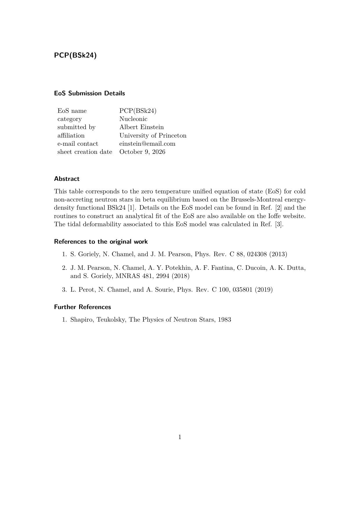
In addition to the CompOSE tables, the contributor should also provide a data sheet. Python interfaces have been developed that will allow the contributor to provide the required information, from which the PDF document will be automatically created from a \(\LaTeX\) template. Each of the required information will be described in turn.
A brief description of the EoS, such as key physical inputs along with any methods that were used to create it, can be provided in the abstract. Note that you can provide \(\LaTeX\) symbols by using the $ symbol, while \(\LaTeX\) commands must be proceeded with an additional backslash \ so that Python does not try and interpret these as Python syntax. For example, one should use \\textbf instead of \textbf. Supplementary references can be provided, but this is not
mandatory.
[35]:
from compytools import (
    DataSheet,
    SubmissionDetails,
    NuclearMatterProperties,
    NeutronStarProperties
)

# We truncate the original abstract for the sake of clarity
abstract = """
This table corresponds to the zero temperature unified equation of state (EoS)
for cold non-accreting neutron stars in beta equilibrium based on the Brussels-Montreal energy-density
functional BSk24 [1]. Details on the EoS model can be found in Ref. [2] and the routines to
construct an analytical fit of the EoS are also available on the Ioffe website.
The tidal deformability associated to this EoS model was calculated in Ref. [3].
"""

references = {
    1: "S. Goriely, N. Chamel, and J. M. Pearson, Phys. Rev. C 88, 024308 (2013)",
    2: "J. M. Pearson, N. Chamel, A. Y. Potekhin, A. F. Fantina, C. Ducoin, A. K. Dutta, and S. Goriely, MNRAS 481, 2994 (2018)",
    3: "L. Perot, N. Chamel, and A. Sourie, Phys. Rev. C 100, 035801 (2019)"
}

further_refs = {
    1: "Shapiro, Teukolsky, The Physics of Neutron Stars, 1983"
}
The contributor can provide details of the submitting author as well as the name of the EoS as follows:
[36]:
submission_details = SubmissionDetails(
    eos_name='PCP(BSk24)',
    category='Nucleonic',
    submitted_by='Albert Einstein',
    affiliation='University of Princeton',
    email='einstein@email.com',
    abstract=abstract,
)
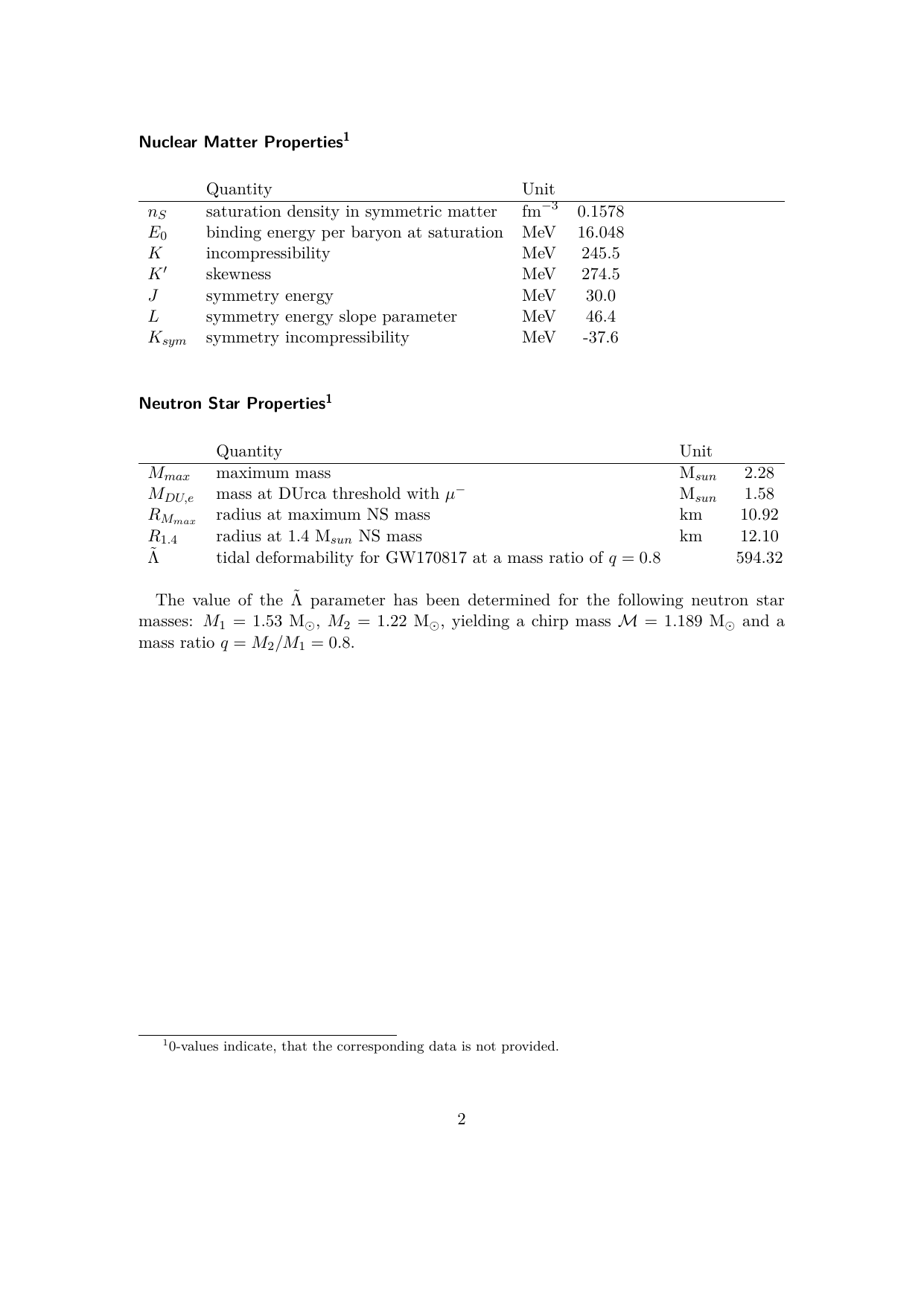
while the nuclear empirical parameters associated with the EoS should be provided via the NuclearMatterProperties class:
[37]:
nuclear_params = NuclearMatterProperties(
    saturation_density_ns=0.1578,
    binding_energy_per_baryon_at_sat_E0=16.048,
    isoscalar_incompressibility_modulus_K=245.5,
    minus_isoscalar_skewness_Kprime=274.5,
    symmetry_energy_J=30.0,
    symmetry_energy_slope_param_L=46.4,
    symmetry_incompressibility_Ksym=-37.6
)
The arguments to NuclearMatterProperties correspond to the following mathematical notation:
Argument |
Notation |
|---|---|
|
\(n_{s}\) |
|
\(E_{0}\) |
|
\(K\) |
|
\(K^{\prime}\) |
|
\(J\) |
|
\(L\) |
|
\(K_{sym}\) |
CompOSE uses the convention that \(E_{0}\) should be positive. If possible, the user should provide the isoscalar parameters to at least second order. If either of these criteria are not met, then ComPyTools will show a warning message.
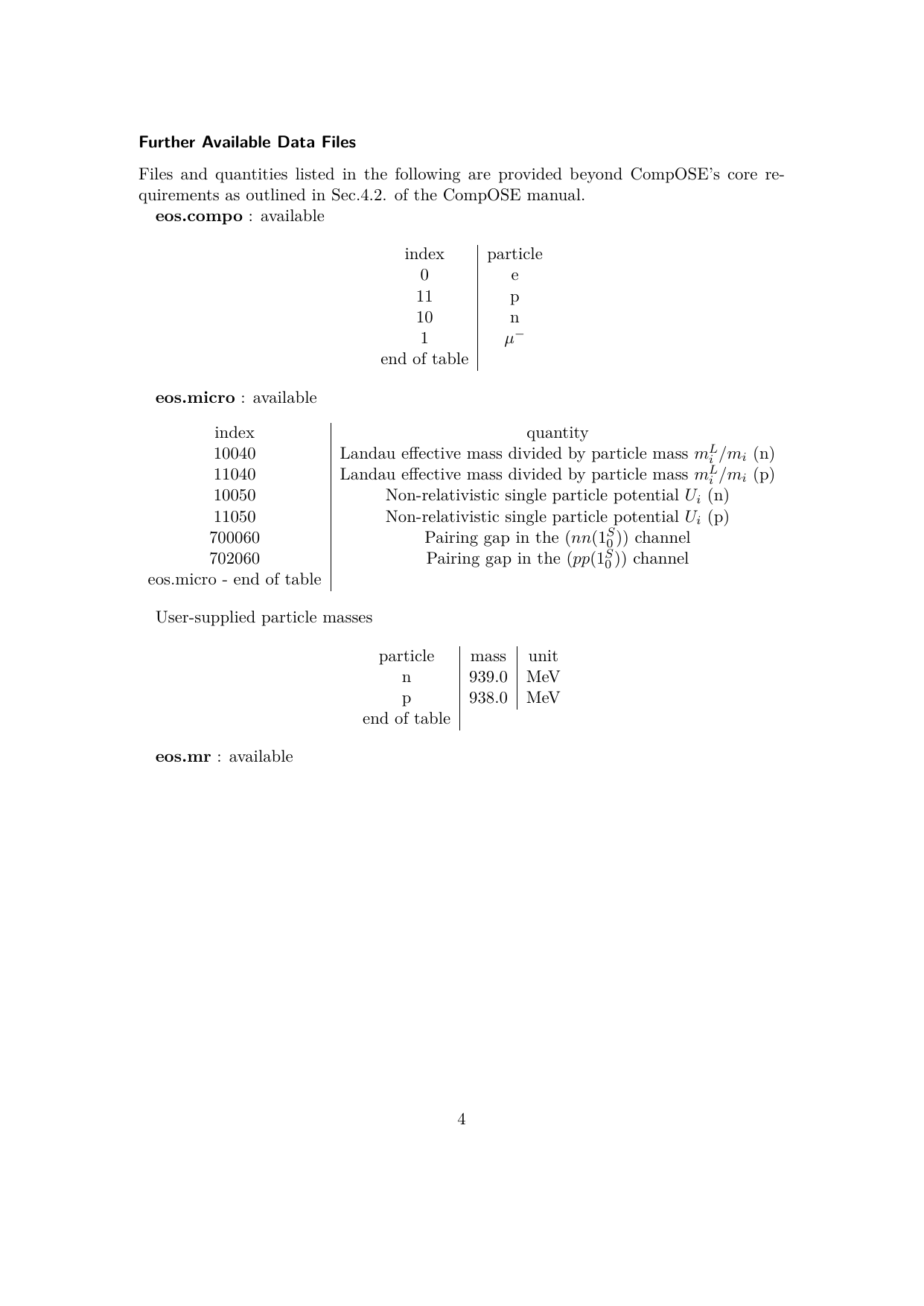
If the contributor has used particle masses that differ from values provided via the Particle Data Group dataset, then they can supply their values as follows:
[38]:
particle_masses = {
    'neutron': 939.0,
    'proton': 938.0,
}
where particle masses should be given in MeV.
Finally, the information is combined using the DataSheet class and the PDF is generated using the .write() method. Note that the neutron star static properties can be provided via ns_data that was generated previously via the NeutronStarData class above.
[39]:
sheet = DataSheet(
    eos=eos,
    submission_details=submission_details,
    nuclear_matter=nuclear_params,
    neutron_star_data=ns_data,
    references=references,
    further_references=further_refs,
    particle_masses=particle_masses
)

content = sheet.write(tmpdir.name)
[11:45:39] INFO Successfully wrote data sheet to: /tmp/tmpog8img1n. datasheet.py:340
The further_references and the particle_masses arguments are not mandatory and can be omitted if not used.
[40]:
from pdf2image import convert_from_path
from IPython.display import display

# Allows us to display the PDF document within the documentation.
datasheet_path = os.path.join(tmpdir.name, 'datasheet.pdf')
pages = convert_from_path(datasheet_path, dpi=150)
for page in pages:
    display(page)
Once all of the CompOSE files and the data sheet have been created, you can arrange to have the data added to the CompOSE web site by contacting the CompOSE core team at the following e-mail address: develop.compose@obspm.fr.